Load libraries
library(Seurat)
library(knitr)
library(kableExtra)
Load the Seurat object from part 1
load(file="original_seurat_object.RData")
experiment.aggregate
## An object of class Seurat
## 12811 features across 2896 samples within 1 assay
## Active assay: RNA (12811 features)
Some basic QA/QC of the metadata, print tables of the 5% quantiles.
Show 5% quantiles for number of genes per cell per sample
do.call("cbind", tapply(experiment.aggregate$nFeature_RNA, Idents(experiment.aggregate),quantile,probs=seq(0,1,0.05)))
##      UCD_Adj_VitE UCD_Supp_VitE UCD_VitE_Def
## 0%         200.00        246.00       235.00
## 5%         357.15        383.00       381.30
## 10%        418.50        488.90       475.20
## 15%        566.95        592.40       642.90
## 20%        847.00        740.00       787.00
## 25%       1005.50        829.50       933.50
## 30%       1102.00        927.10      1062.00
## 35%       1189.05       1003.65      1156.55
## 40%       1301.20       1079.80      1267.40
## 45%       1427.00       1185.75      1428.90
## 50%       1584.50       1302.50      1555.50
## 55%       1689.30       1423.45      1671.15
## 60%       1814.00       1555.20      1810.00
## 65%       1934.70       1661.05      1907.00
## 70%       2099.00       1805.80      2038.40
## 75%       2250.00       1954.00      2172.50
## 80%       2470.80       2063.40      2336.40
## 85%       2763.55       2287.05      2578.35
## 90%       3001.00       2514.30      2928.90
## 95%       3306.05       2801.20      3319.40
## 100%      4514.00       4238.00      4735.00
Show 5% quantiles for number of UMI per cell per sample
do.call("cbind", tapply(experiment.aggregate$nCount_RNA, Idents(experiment.aggregate),quantile,probs=seq(0,1,0.05)))
##      UCD_Adj_VitE UCD_Supp_VitE UCD_VitE_Def
## 0%         496.00        498.00       499.00
## 5%         551.15        565.95       586.00
## 10%        693.50        673.90       712.30
## 15%        866.90        816.85       894.65
## 20%       1287.80       1062.40      1164.60
## 25%       1623.00       1209.25      1401.25
## 30%       1873.50       1397.90      1690.00
## 35%       2067.00       1571.65      1898.55
## 40%       2282.40       1776.60      2165.60
## 45%       2649.00       2013.25      2581.60
## 50%       3036.00       2231.00      2893.00
## 55%       3390.85       2521.10      3278.10
## 60%       3785.40       2834.40      3647.60
## 65%       4142.45       3239.60      4168.00
## 70%       4622.80       3673.50      4563.00
## 75%       5297.25       4242.75      5018.25
## 80%       6229.80       4693.20      5677.40
## 85%       7924.55       5442.35      6890.60
## 90%       9066.50       6447.30      8489.90
## 95%      10963.05       7869.40     11031.10
## 100%     20634.00      19948.00     26952.00
Show 5% quantiles for number of mitochondrial percentage per cell per sample
round(do.call("cbind", tapply(experiment.aggregate$percent.mito, Idents(experiment.aggregate),quantile,probs=seq(0,1,0.05))), digits = 3)
##      UCD_Adj_VitE UCD_Supp_VitE UCD_VitE_Def
## 0%          0.031         0.000        0.000
## 5%          1.354         0.653        0.652
## 10%         2.059         0.991        1.105
## 15%         2.461         1.409        1.536
## 20%         2.842         1.693        1.794
## 25%         3.179         1.972        2.121
## 30%         3.548         2.215        2.411
## 35%         3.844         2.598        2.718
## 40%         4.233         2.904        3.023
## 45%         4.526         3.152        3.399
## 50%         4.908         3.429        3.749
## 55%         5.346         3.825        4.111
## 60%         5.666         4.209        4.482
## 65%         6.023         4.662        4.856
## 70%         6.482         5.018        5.297
## 75%         6.996         5.483        5.834
## 80%         7.586         5.980        6.497
## 85%         8.356         6.626        7.157
## 90%        10.026         7.529        8.059
## 95%        27.560        10.056       10.858
## 100%       59.279        51.836       64.441
Table of cell cycle
table(experiment.aggregate@meta.data$cell.cycle) %>% kable(caption = "Number of Cells in each Cell Cycle Stage", col.names = c("Stage", "Count"), align = "c") %>% kable_styling()
| Stage | Count |
|---|---|
| G1 | 2764 |
| G2M | 97 |
| S | 35 |
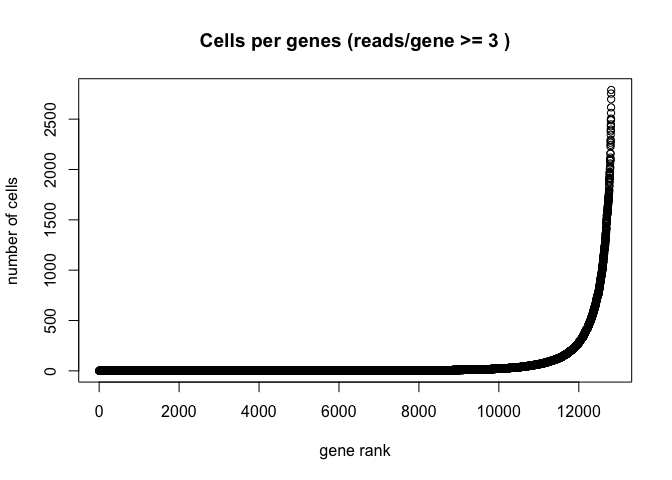
Plot the number of cells each gene is represented by
plot(sort(Matrix::rowSums(GetAssayData(experiment.aggregate) >= 3)) , xlab="gene rank", ylab="number of cells", main="Cells per genes (reads/gene >= 3 )")
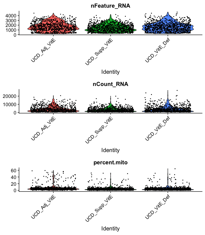
Violin plot of 1) number of genes, 2) number of UMI and 3) percent mitochondrial genes
VlnPlot(
  experiment.aggregate,
  features = c("nFeature_RNA", "nCount_RNA","percent.mito"),
  ncol = 1, pt.size = 0.3)
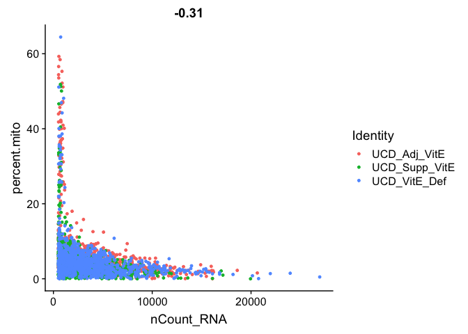
Gene Plot, scatter plot of gene expression across cells, (colored by sample)
FeatureScatter(experiment.aggregate, feature1 = "nCount_RNA", feature2 = "percent.mito")
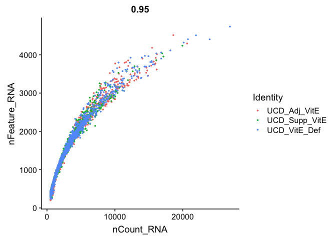
FeatureScatter(
  experiment.aggregate, "nCount_RNA", "nFeature_RNA",
  pt.size = 0.5)
Cell filtering
We use the information above to filter out cells. Here we choose those that have percent mitochondrial genes max of 10% and unique UMI counts under 20,000 or greater than 500.
experiment.aggregate <- subset(experiment.aggregate, percent.mito <= 10)

experiment.aggregate <- subset(experiment.aggregate, nCount_RNA >= 500 & nCount_RNA <= 20000)

experiment.aggregate
## An object of class Seurat
## 12811 features across 2681 samples within 1 assay
## Active assay: RNA (12811 features)
You may also want to filter out additional genes.
When creating the base Seurat object we did filter out some genes, recall Keep all genes expressed in >= 10 cells. After filtering cells and you may want to be more aggressive with the gene filter. Seurat doesn’t supply such a function (that I can find), so below is a function that can do so, it filters genes requiring a min.value (log-normalized) in at least min.cells, here expression of 1 in at least 400 cells.
FilterGenes <-
 function (object, min.value=1, min.cells = 0, genes = NULL) {
   genes.use <- rownames(object)
   if (!is.null(genes)) {
     genes.use <- intersect(genes.use, genes)
     object@data <- GetAssayData(object)[genes.use, ]
   } else if (min.cells > 0) {
     num.cells <- Matrix::rowSums(GetAssayData(object) > min.value)
     genes.use <- names(num.cells[which(num.cells >= min.cells)])
     object = object[genes.use, ]
   }
  object <- LogSeuratCommand(object = object)
  return(object)
}

experiment.aggregate.genes <- FilterGenes(object = experiment.aggregate, min.value = 1, min.cells = 400)
experiment.aggregate.genes
## An object of class Seurat
## 1117 features across 2681 samples within 1 assay
## Active assay: RNA (1117 features)
table(experiment.aggregate$orig.ident)
##
##  UCD_Adj_VitE UCD_Supp_VitE  UCD_VitE_Def
##           808           947           926
Next we want to normalize the data
After filtering out cells from the dataset, the next step is to normalize the data. By default, we employ a global-scaling normalization method LogNormalize that normalizes the gene expression measurements for each cell by the total expression, multiplies this by a scale factor (10,000 by default), and then log-transforms the data.
?NormalizeData
experiment.aggregate <- NormalizeData(
  object = experiment.aggregate,
  normalization.method = "LogNormalize",
  scale.factor = 10000)
Identify variable genes
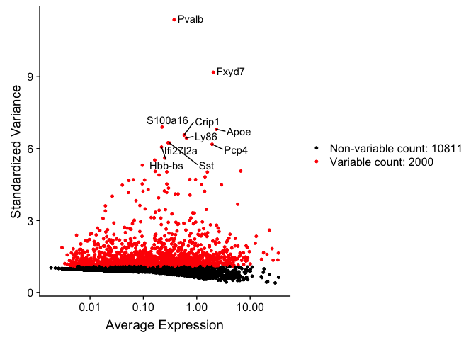
The function FindVariableFeatures identifies the most highly variable genes (default 2000 genes) by fitting a line to the relationship of log(variance) and log(mean) using loess smoothing, uses this information to standardize the data, then calculates the variance of the standardized data. This helps avoid selecting genes that only appear variable due to their expression level.
?FindVariableFeatures

experiment.aggregate <- FindVariableFeatures(
  object = experiment.aggregate,
  selection.method = "vst")

length(VariableFeatures(experiment.aggregate))
## [1] 2000
top10 <- head(VariableFeatures(experiment.aggregate), 10)

top10
##  [1] "Pvalb"    "Fxyd7"    "S100a16"  "Apoe"     "Crip1"    "Ly86"
##  [7] "Ifi27l2a" "Sst"      "Pcp4"     "Hbb-bs"
vfp1 <- VariableFeaturePlot(experiment.aggregate)
vfp1 <- LabelPoints(plot = vfp1, points = top10, repel = TRUE)
vfp1
Question(s)
- Play some with the filtering parameters, see how results change?
- How do the results change if you use selection.method = “dispersion” or selection.method = “mean.var.plot”
Finally, lets save the filtered and normalized data
save(experiment.aggregate, file="pre_sample_corrected.RData")
Get the next Rmd file
download.file("https://raw.githubusercontent.com/ucdavis-bioinformatics-training/2019-single-cell-RNA-sequencing-Workshop-UCD_UCSF/master/scrnaseq_analysis/scRNA_Workshop-PART3.Rmd", "scRNA_Workshop-PART3.Rmd")
Session Information
sessionInfo()
## R version 3.6.0 (2019-04-26)
## Platform: x86_64-apple-darwin15.6.0 (64-bit)
## Running under: macOS Mojave 10.14.5
##
## Matrix products: default
## BLAS:   /Library/Frameworks/R.framework/Versions/3.6/Resources/lib/libRblas.0.dylib
## LAPACK: /Library/Frameworks/R.framework/Versions/3.6/Resources/lib/libRlapack.dylib
##
## locale:
## [1] en_US.UTF-8/en_US.UTF-8/en_US.UTF-8/C/en_US.UTF-8/en_US.UTF-8
##
## attached base packages:
## [1] stats     graphics  grDevices utils     datasets  methods   base
##
## other attached packages:
## [1] kableExtra_1.1.0 knitr_1.23       Seurat_3.0.2
##
## loaded via a namespace (and not attached):
##  [1] nlme_3.1-140        tsne_0.1-3          bitops_1.0-6
##  [4] webshot_0.5.1       RColorBrewer_1.1-2  httr_1.4.0
##  [7] sctransform_0.2.0   tools_3.6.0         R6_2.4.0
## [10] irlba_2.3.3         KernSmooth_2.23-15  lazyeval_0.2.2
## [13] colorspace_1.4-1    withr_2.1.2         npsurv_0.4-0
## [16] tidyselect_0.2.5    gridExtra_2.3       compiler_3.6.0
## [19] rvest_0.3.4         xml2_1.2.0          plotly_4.9.0
## [22] labeling_0.3        caTools_1.17.1.2    scales_1.0.0
## [25] lmtest_0.9-37       readr_1.3.1         ggridges_0.5.1
## [28] pbapply_1.4-0       stringr_1.4.0       digest_0.6.19
## [31] rmarkdown_1.13      R.utils_2.9.0       pkgconfig_2.0.2
## [34] htmltools_0.3.6     bibtex_0.4.2        highr_0.8
## [37] htmlwidgets_1.3     rlang_0.3.4         rstudioapi_0.10
## [40] zoo_1.8-6           jsonlite_1.6        ica_1.0-2
## [43] gtools_3.8.1        dplyr_0.8.1         R.oo_1.22.0
## [46] magrittr_1.5        Matrix_1.2-17       Rcpp_1.0.1
## [49] munsell_0.5.0       ape_5.3             reticulate_1.12
## [52] R.methodsS3_1.7.1   stringi_1.4.3       yaml_2.2.0
## [55] gbRd_0.4-11         MASS_7.3-51.4       gplots_3.0.1.1
## [58] Rtsne_0.15          plyr_1.8.4          grid_3.6.0
## [61] parallel_3.6.0      gdata_2.18.0        listenv_0.7.0
## [64] ggrepel_0.8.1       crayon_1.3.4        lattice_0.20-38
## [67] cowplot_0.9.4       splines_3.6.0       hms_0.4.2
## [70] SDMTools_1.1-221.1  pillar_1.4.1        igraph_1.2.4.1
## [73] future.apply_1.3.0  reshape2_1.4.3      codetools_0.2-16
## [76] glue_1.3.1          evaluate_0.14       lsei_1.2-0
## [79] metap_1.1           data.table_1.12.2   png_0.1-7
## [82] Rdpack_0.11-0       gtable_0.3.0        RANN_2.6.1
## [85] purrr_0.3.2         tidyr_0.8.3         future_1.13.0
## [88] assertthat_0.2.1    ggplot2_3.2.0       xfun_0.7
## [91] rsvd_1.0.1          survival_2.44-1.1   viridisLite_0.3.0
## [94] tibble_2.1.3        cluster_2.1.0       globals_0.12.4
## [97] fitdistrplus_1.0-14 ROCR_1.0-7