Load libraries
library(Seurat)
Load the Seurat object
load(file="pre_sample_corrected.RData")
experiment.aggregate
## An object of class Seurat
## 12811 features across 2681 samples within 1 assay
## Active assay: RNA (12811 features)
experiment.test <- experiment.aggregate
set.seed(12345)
rand.genes <- sample(1:nrow(experiment.test), 500,replace = F)
mat <- as.matrix(GetAssayData(experiment.test, slot="data"))
mat[rand.genes,experiment.test$batchid=="Batch2"] <- mat[rand.genes,experiment.test$batchid=="Batch2"] + 0.18
experiment.test = SetAssayData(experiment.test, slot="data", new.data= mat )
Exploring Batch effects 3 ways, none, Seurat [vars.to.regress] and COMBAT
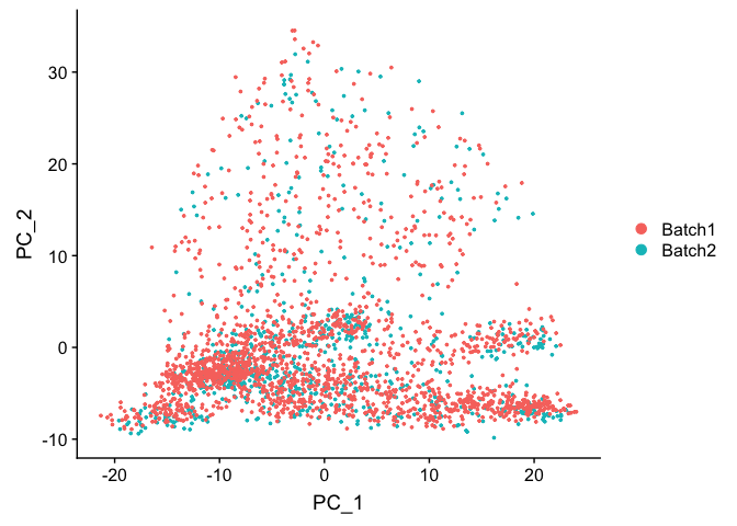
First lets view the data without any corrections
PCA in prep for tSNE
ScaleData - Scales and centers genes in the dataset.
?ScaleData
experiment.test.noc <- ScaleData(object = experiment.test)
## Centering and scaling data matrix
Run PCA
experiment.test.noc <- RunPCA(object = experiment.test.noc)
## PC_ 1
## Positive:  Txn1, Sncg, Fez1, S100a10, Atp6v0b, Lxn, Dctn3, Tppp3, Sh3bgrl3, Rabac1
## 	   Cisd1, Ppia, Fxyd2, Atp6v1f, Stmn3, Ndufa11, Atp5g1, Bex2, Atpif1, Uchl1
## 	   Ndufa4, Psmb6, Ubb, Hagh, Anxa2, Gabarapl2, Rgs10, Nme1, Prdx2, Psmb3
## Negative:  Mt1, Malat1, Adcyap1, Ptn, Apoe, Zeb2, Mt2, Timp3, Fabp7, Gpm6b
## 	   Gal, Kit, Qk, Plp1, Atp2b4, Ifitm3, 6330403K07Rik, Sparc, Id3, Gap43
## 	   Selenop, Gpx3, Zfp36l1, Rgcc, Scg2, Cbfb, Zfp36, Igfbp7, Marcksl1, Phlda1
## PC_ 2
## Positive:  Nefh, Cntn1, Thy1, S100b, Sv2b, Cplx1, Slc17a7, Vamp1, Nefm, Lynx1
## 	   Endod1, Scn1a, Atp1b1, Vsnl1, Nat8l, Ntrk3, Sh3gl2, Fam19a2, Eno2, Scn1b
## 	   Spock1, Scn8a, Glrb, Syt2, Scn4b, Lrrn1, Lgi3, Snap25, Atp2b2, Cpne6
## Negative:  Malat1, Cd24a, Tmem233, Cd9, Dusp26, Mal2, Carhsp1, Tmem158, Fxyd2, Ctxn3
## 	   Prkca, Ubb, Crip2, Arpc1b, Gna14, S100a6, Cd44, Tmem45b, Klf5, Tceal9
## 	   Cd82, Hs6st2, Bex3, Emp3, Ift122, Fam89a, Pfn1, Dynll1, Acpp, Smim5
## PC_ 3
## Positive:  P2ry1, Fam19a4, Gm7271, Rarres1, Th, Zfp521, Wfdc2, Tox3, Gfra2, D130079A08Rik
## 	   Iqsec2, Pou4f2, Rgs5, Kcnd3, Id4, Rasgrp1, Slc17a8, Casz1, Cdkn1a, Piezo2
## 	   Dpp10, Gm11549, Fxyd6, Spink2, Rgs10, Zfhx3, C1ql4, Cd34, Gabra1, Cckar
## Negative:  Calca, Basp1, Gap43, Ppp3ca, Map1b, Scg2, Cystm1, Tmem233, Calm1, Map7d2
## 	   Ift122, Tubb3, Ncdn, Resp18, Prkca, Etv1, Nmb, Skp1a, Crip2, Camk2a
## 	   Epb41l3, Tspan8, Ntrk1, Deptor, Gna14, Adk, Jak1, Tmem255a, Etl4, Camk2g
## PC_ 4
## Positive:  Id3, Timp3, Selenop, Pvalb, Ifitm3, Sparc, Igfbp7, Adk, Sgk1, Tm4sf1
## 	   Ly6c1, Id1, Etv1, Nsg1, Mt2, Slc17a7, Zfp36l1, Cldn5, Spp1, Ier2
## 	   Aldoc, Shox2, Cxcl12, Ptn, Itm2a, Qk, Stxbp6, Sparcl1, Jak1, Slit2
## Negative:  Gap43, Calca, Stmn1, Tac1, Ppp3ca, 6330403K07Rik, Arhgdig, Alcam, Adcyap1, Prune2
## 	   Kit, Ngfr, Ywhag, Gal, Fxyd6, Atp1a1, Smpd3, Ntrk1, Tmem100, Cd24a
## 	   Atp2b4, Mt3, Cnih2, Tppp3, Gpx3, S100a11, Scn7a, Snap25, Cbfb, Gnb1
## PC_ 5
## Positive:  Cpne3, Klf5, Acpp, Fxyd2, Jak1, Nppb, Rgs4, Osmr, Zfhx3, Nbl1
## 	   Etv1, Htr1f, Gm525, Sst, Adk, Tspan8, Cysltr2, Parm1, Tmem233, Prkca
## 	   Cd24a, Npy2r, Prune2, Nts, Socs2, Dgkz, Gnb1, Phf24, Il31ra, Plxnc1
## Negative:  Mt1, Ptn, B2m, Prdx1, Dbi, Mt3, Ifitm3, Fxyd7, Id3, Mt2
## 	   Calca, S100a16, Sparc, Pcp4l1, Ifitm2, Selenop, Igfbp7, Rgcc, Hspb1, Selenom
## 	   Abcg2, S100a13, Apoe, Tm4sf1, Timp3, Itm2a, Ubb, Ly6c1, Cryab, Cebpd
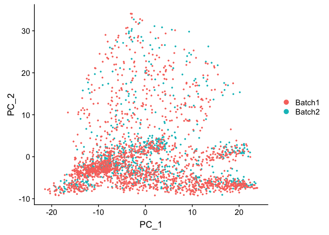
DimPlot(object = experiment.test.noc, group.by = "batchid", reduction = "pca")
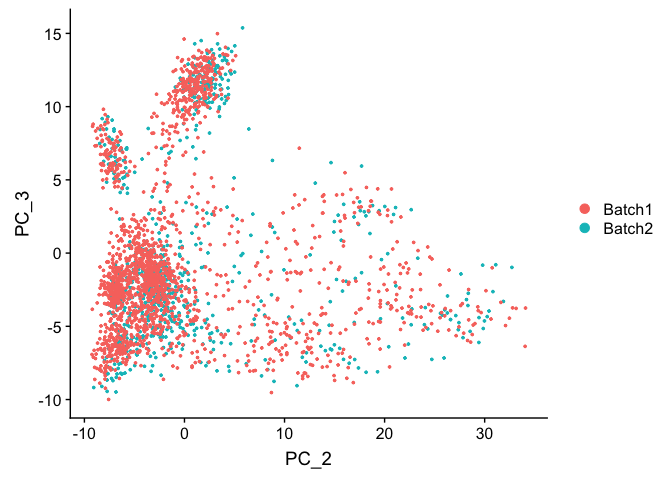
DimPlot(object = experiment.test.noc, group.by = "batchid", dims = c(2,3), reduction = "pca")
PCA Elbow plot to determine how many principal components to use in downstream analyses. Components after the “elbow” in the plot generally explain little additional variability in the data.
ElbowPlot(experiment.test.noc)
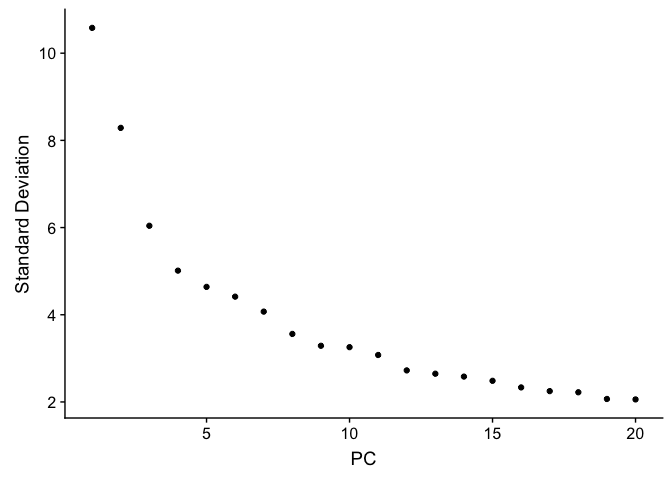
We use 10 components in downstream analyses. Using more components more closely approximates the full data set but increases run time.
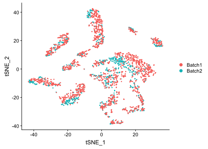
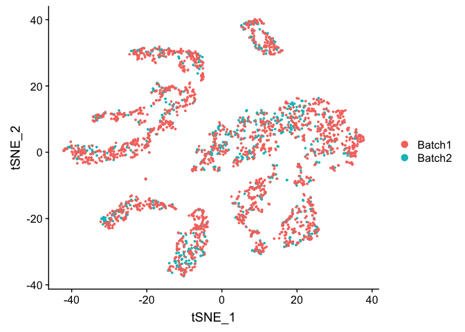
TSNE Plot
pcs.use <- 10
experiment.test.noc <- RunTSNE(object = experiment.test.noc, dims = 1:pcs.use)
DimPlot(object = experiment.test.noc,  group.by = "batchid")
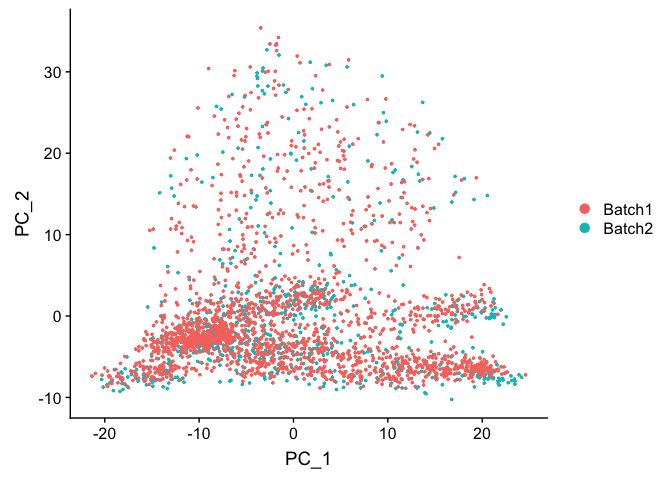
Correct for sample to sample differences (seurat)
Use vars.to.regress to correct for the sample to sample differences and percent mitochondria
experiment.test.regress <- ScaleData(object = experiment.test,
                    vars.to.regress = c("batchid"), model.use = "linear")
## Regressing out batchid
## Centering and scaling data matrix
experiment.test.regress <- RunPCA(object =experiment.test.regress)
## PC_ 1
## Positive:  Txn1, Sncg, Fez1, S100a10, Atp6v0b, Lxn, Dctn3, Tppp3, Sh3bgrl3, Rabac1
## 	   Cisd1, Ppia, Fxyd2, Atp6v1f, Stmn3, Ndufa11, Atp5g1, Bex2, Atpif1, Uchl1
## 	   Ndufa4, Psmb6, Ubb, Hagh, Anxa2, Gabarapl2, Rgs10, Nme1, Prdx2, Psmb3
## Negative:  Mt1, Malat1, Adcyap1, Ptn, Apoe, Zeb2, Mt2, Timp3, Fabp7, Gpm6b
## 	   Gal, Kit, Qk, Atp2b4, Plp1, Ifitm3, 6330403K07Rik, Sparc, Id3, Gap43
## 	   Gpx3, Selenop, Zfp36l1, Rgcc, Scg2, Cbfb, Zfp36, Igfbp7, Marcksl1, Phlda1
## PC_ 2
## Positive:  Nefh, Cntn1, Thy1, S100b, Sv2b, Cplx1, Slc17a7, Vamp1, Nefm, Lynx1
## 	   Endod1, Atp1b1, Scn1a, Nat8l, Vsnl1, Ntrk3, Sh3gl2, Fam19a2, Eno2, Scn1b
## 	   Spock1, Scn8a, Glrb, Syt2, Scn4b, Lrrn1, Atp2b2, Lgi3, Cpne6, Snap25
## Negative:  Malat1, Cd24a, Tmem233, Cd9, Dusp26, Mal2, Tmem158, Carhsp1, Fxyd2, Ctxn3
## 	   Ubb, Prkca, Arpc1b, Crip2, S100a6, Gna14, Cd44, Tmem45b, Klf5, Tceal9
## 	   Bex3, Hs6st2, Cd82, Emp3, Pfn1, Ift122, Tubb2b, Fam89a, Dynll1, Gadd45g
## PC_ 3
## Positive:  P2ry1, Fam19a4, Gm7271, Rarres1, Th, Zfp521, Wfdc2, Tox3, Gfra2, D130079A08Rik
## 	   Iqsec2, Pou4f2, Rgs5, Kcnd3, Id4, Rasgrp1, Slc17a8, Casz1, Cdkn1a, Piezo2
## 	   Dpp10, Gm11549, Fxyd6, Rgs10, Spink2, Zfhx3, C1ql4, Cd34, Gabra1, Cckar
## Negative:  Calca, Basp1, Gap43, Ppp3ca, Map1b, Scg2, Cystm1, Tmem233, Map7d2, Calm1
## 	   Ift122, Tubb3, Ncdn, Resp18, Prkca, Etv1, Nmb, Skp1a, Crip2, Epb41l3
## 	   Camk2a, Ntrk1, Tspan8, Deptor, Gna14, Adk, Jak1, Tmem255a, Etl4, Camk2g
## PC_ 4
## Positive:  Id3, Timp3, Selenop, Pvalb, Ifitm3, Sparc, Igfbp7, Adk, Tm4sf1, Ly6c1
## 	   Sgk1, Id1, Etv1, Nsg1, Mt2, Cldn5, Zfp36l1, Ier2, Itm2a, Spp1
## 	   Slc17a7, Aldoc, Ptn, Cxcl12, Shox2, Qk, Stxbp6, Sparcl1, Slit2, Jak1
## Negative:  Gap43, Calca, Stmn1, Tac1, Ppp3ca, Arhgdig, 6330403K07Rik, Alcam, Prune2, Adcyap1
## 	   Kit, Ngfr, Ywhag, Atp1a1, Fxyd6, Gal, Smpd3, Ntrk1, Tmem100, Cd24a
## 	   Atp2b4, Mt3, Cnih2, Tppp3, Scn7a, Gpx3, S100a11, Snap25, Gnb1, Cbfb
## PC_ 5
## Positive:  Cpne3, Klf5, Jak1, Acpp, Fxyd2, Nppb, Osmr, Gm525, Htr1f, Sst
## 	   Etv1, Nbl1, Rgs4, Zfhx3, Cysltr2, Adk, Tspan8, Npy2r, Nts, Parm1
## 	   Tmem233, Prkca, Cd24a, Socs2, Prune2, Il31ra, Dgkz, Ptafr, Gnb1, Ptprk
## Negative:  Mt1, Ptn, B2m, Dbi, Prdx1, Mt3, Fxyd7, Ifitm3, S100a16, Calca
## 	   Id3, Mt2, Pcp4l1, Sparc, Selenop, Ifitm2, Rgcc, Igfbp7, Abcg2, Tm4sf1
## 	   Apoe, Selenom, S100a13, Cryab, Hspb1, Timp3, Gap43, Ubb, Ly6c1, Phlda1
DimPlot(object = experiment.test.regress, group.by = "batchid", reduction.use = "pca")
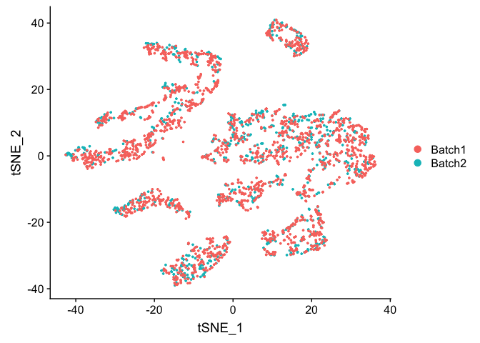
Corrected TSNE Plot
experiment.test.regress <- RunTSNE(object = experiment.test.regress, dims.use = 1:pcs.use)
DimPlot(object = experiment.test.regress, group.by = "batchid", reduction = "tsne")
COMBAT corrected, https://academic.oup.com/biostatistics/article-lookup/doi/10.1093/biostatistics/kxj037
library(sva)
## Loading required package: mgcv
## Loading required package: nlme
## This is mgcv 1.8-28. For overview type 'help("mgcv-package")'.
## Loading required package: genefilter
## Loading required package: BiocParallel
?ComBat
m = as.matrix(GetAssayData(experiment.test))
com = ComBat(dat=m, batch=as.numeric(as.factor(experiment.test$orig.ident)), prior.plots=FALSE, par.prior=TRUE)
## Found3batches
## Adjusting for0covariate(s) or covariate level(s)
## Standardizing Data across genes
## Fitting L/S model and finding priors
## Finding parametric adjustments
## Adjusting the Data
experiment.test.combat <- experiment.test
experiment.test.combat <- SetAssayData(experiment.test.combat, new.data = as.matrix(com))
experiment.test.combat = ScaleData(experiment.test.combat)
## Centering and scaling data matrix
Principal components on ComBat adjusted data
experiment.test.combat <- RunPCA(object = experiment.test.combat)
## PC_ 1
## Positive:  Txn1, Sncg, Fez1, S100a10, Atp6v0b, Lxn, Dctn3, Tppp3, Sh3bgrl3, Rabac1
## 	   Cisd1, Ppia, Stmn3, Fxyd2, Ndufa11, Atp6v1f, Atp5g1, Bex2, Atpif1, Uchl1
## 	   Ndufa4, Psmb6, Ubb, Anxa2, Gabarapl2, Hagh, Nme1, Psmb3, Rgs10, Prdx2
## Negative:  Mt1, Malat1, Adcyap1, Ptn, Apoe, Zeb2, Mt2, Timp3, Fabp7, Gal
## 	   Gpm6b, Kit, Qk, Atp2b4, Plp1, Ifitm3, 6330403K07Rik, Sparc, Id3, Gpx3
## 	   Selenop, Gap43, Zfp36l1, Rgcc, Scg2, Cbfb, Zfp36, Igfbp7, Marcksl1, Phlda1
## PC_ 2
## Positive:  Nefh, Cntn1, Thy1, Sv2b, S100b, Slc17a7, Cplx1, Vamp1, Nefm, Lynx1
## 	   Endod1, Atp1b1, Scn1a, Nat8l, Vsnl1, Ntrk3, Scn8a, Sh3gl2, Fam19a2, Eno2
## 	   Scn1b, Spock1, Glrb, Syt2, Scn4b, Cpne6, Lgi3, Lrrn1, Atp2b2, Clec2l
## Negative:  Malat1, Cd24a, Tmem233, Cd9, Dusp26, Mal2, Tmem158, Carhsp1, Fxyd2, Ubb
## 	   Ctxn3, Crip2, Arpc1b, Prkca, S100a6, Gna14, Cd44, Tmem45b, Klf5, Tceal9
## 	   Bex3, Hs6st2, Cd82, Emp3, Pfn1, Tubb2b, Dynll1, Ift122, Fam89a, Acpp
## PC_ 3
## Positive:  P2ry1, Fam19a4, Gm7271, Rarres1, Th, Zfp521, Wfdc2, Tox3, Gfra2, D130079A08Rik
## 	   Iqsec2, Pou4f2, Rgs5, Kcnd3, Rasgrp1, Id4, Slc17a8, Casz1, Cdkn1a, Piezo2
## 	   Dpp10, Gm11549, Fxyd6, Rgs10, Zfhx3, Spink2, C1ql4, Gabra1, Cd34, Synpr
## Negative:  Calca, Basp1, Gap43, Ppp3ca, Map1b, Scg2, Cystm1, Tmem233, Map7d2, Ift122
## 	   Calm1, Ncdn, Tubb3, Prkca, Resp18, Etv1, Skp1a, Nmb, Crip2, Camk2a
## 	   Tspan8, Epb41l3, Ntrk1, Gna14, Deptor, Adk, Jak1, Tmem255a, Etl4, Dusp26
## PC_ 4
## Positive:  Id3, Timp3, Pvalb, Selenop, Sparc, Adk, Ifitm3, Igfbp7, Etv1, Nsg1
## 	   Sgk1, Tm4sf1, Id1, Ly6c1, Mt2, Spp1, Slc17a7, Zfp36l1, Shox2, Ier2
## 	   Aldoc, Cldn5, Itm2a, Ptn, Jak1, Qk, Cxcl12, Stxbp6, Tspan8, Slit2
## Negative:  Gap43, Calca, Stmn1, Tac1, Arhgdig, Ppp3ca, 6330403K07Rik, Alcam, Adcyap1, Prune2
## 	   Ngfr, Kit, Ywhag, Atp1a1, Gal, Fxyd6, Smpd3, Ntrk1, Tmem100, Mt3
## 	   Atp2b4, Cd24a, Cnih2, Tppp3, S100a11, Gpx3, Scn7a, Cbfb, Snap25, Gnb1
## PC_ 5
## Positive:  Cpne3, Klf5, Acpp, Fxyd2, Jak1, Nppb, Osmr, Nbl1, Gm525, Htr1f
## 	   Rgs4, Sst, Etv1, Zfhx3, Cysltr2, Tspan8, Adk, Npy2r, Parm1, Tmem233
## 	   Cd24a, Nts, Prkca, Prune2, Socs2, Il31ra, Gnb1, Dgkz, Phf24, Ptafr
## Negative:  Mt1, Ptn, B2m, Dbi, Prdx1, Mt3, Id3, Ifitm3, S100a16, Fxyd7
## 	   Mt2, Calca, Sparc, Selenop, Pcp4l1, Ifitm2, Rgcc, Apoe, Cryab, Igfbp7
## 	   Selenom, Ubb, Abcg2, Tm4sf1, Timp3, S100a13, Hspb1, Phlda1, Hspa1a, Dad1
DimPlot(object = experiment.test.combat, group.by = "batchid", reduction = "pca")
TSNE plot on ComBat adjusted data
experiment.test.combat <- RunTSNE(object = experiment.test.combat, dims.use = 1:pcs.use)
DimPlot(object = experiment.test.combat, group.by = "batchid", reduction = "tsne")
Question(s)
- Try a couple of PCA cutoffs (low and high) and compare the TSNE plots from the different methods. Do they look meaningfully different?
Get the next Rmd file
download.file("https://raw.githubusercontent.com/ucdavis-bioinformatics-training/2019-single-cell-RNA-sequencing-Workshop-UCD_UCSF/master/scrnaseq_analysis/scRNA_Workshop-PART4.Rmd", "scRNA_Workshop-PART4.Rmd")
Session Information
sessionInfo()
## R version 3.6.0 (2019-04-26)
## Platform: x86_64-apple-darwin15.6.0 (64-bit)
## Running under: macOS Mojave 10.14.5
##
## Matrix products: default
## BLAS:   /Library/Frameworks/R.framework/Versions/3.6/Resources/lib/libRblas.0.dylib
## LAPACK: /Library/Frameworks/R.framework/Versions/3.6/Resources/lib/libRlapack.dylib
##
## locale:
## [1] en_US.UTF-8/en_US.UTF-8/en_US.UTF-8/C/en_US.UTF-8/en_US.UTF-8
##
## attached base packages:
## [1] stats     graphics  grDevices utils     datasets  methods   base
##
## other attached packages:
## [1] sva_3.32.1          BiocParallel_1.18.0 genefilter_1.66.0
## [4] mgcv_1.8-28         nlme_3.1-140        Seurat_3.0.2
##
## loaded via a namespace (and not attached):
##   [1] tsne_0.1-3           matrixStats_0.54.0   bitops_1.0-6
##   [4] bit64_0.9-7          RColorBrewer_1.1-2   httr_1.4.0
##   [7] sctransform_0.2.0    tools_3.6.0          R6_2.4.0
##  [10] irlba_2.3.3          KernSmooth_2.23-15   DBI_1.0.0
##  [13] BiocGenerics_0.30.0  lazyeval_0.2.2       colorspace_1.4-1
##  [16] npsurv_0.4-0         tidyselect_0.2.5     gridExtra_2.3
##  [19] bit_1.1-14           compiler_3.6.0       Biobase_2.44.0
##  [22] plotly_4.9.0         labeling_0.3         caTools_1.17.1.2
##  [25] scales_1.0.0         lmtest_0.9-37        ggridges_0.5.1
##  [28] pbapply_1.4-0        stringr_1.4.0        digest_0.6.19
##  [31] rmarkdown_1.13       R.utils_2.9.0        pkgconfig_2.0.2
##  [34] htmltools_0.3.6      bibtex_0.4.2         highr_0.8
##  [37] limma_3.40.2         htmlwidgets_1.3      rlang_0.3.4
##  [40] RSQLite_2.1.1        zoo_1.8-6            jsonlite_1.6
##  [43] ica_1.0-2            gtools_3.8.1         dplyr_0.8.1
##  [46] R.oo_1.22.0          RCurl_1.95-4.12      magrittr_1.5
##  [49] Matrix_1.2-17        S4Vectors_0.22.0     Rcpp_1.0.1
##  [52] munsell_0.5.0        ape_5.3              reticulate_1.12
##  [55] R.methodsS3_1.7.1    stringi_1.4.3        yaml_2.2.0
##  [58] gbRd_0.4-11          MASS_7.3-51.4        gplots_3.0.1.1
##  [61] Rtsne_0.15           plyr_1.8.4           blob_1.1.1
##  [64] grid_3.6.0           parallel_3.6.0       gdata_2.18.0
##  [67] listenv_0.7.0        ggrepel_0.8.1        crayon_1.3.4
##  [70] lattice_0.20-38      cowplot_0.9.4        splines_3.6.0
##  [73] annotate_1.62.0      SDMTools_1.1-221.1   knitr_1.23
##  [76] pillar_1.4.1         igraph_1.2.4.1       stats4_3.6.0
##  [79] future.apply_1.3.0   reshape2_1.4.3       codetools_0.2-16
##  [82] XML_3.98-1.20        glue_1.3.1           evaluate_0.14
##  [85] lsei_1.2-0           metap_1.1            data.table_1.12.2
##  [88] png_0.1-7            Rdpack_0.11-0        gtable_0.3.0
##  [91] RANN_2.6.1           purrr_0.3.2          tidyr_0.8.3
##  [94] future_1.13.0        assertthat_0.2.1     ggplot2_3.2.0
##  [97] xfun_0.7             rsvd_1.0.1           xtable_1.8-4
## [100] survival_2.44-1.1    viridisLite_0.3.0    tibble_2.1.3
## [103] IRanges_2.18.1       memoise_1.1.0        AnnotationDbi_1.46.0
## [106] cluster_2.1.0        globals_0.12.4       fitdistrplus_1.0-14
## [109] ROCR_1.0-7