Differential Gene Expression Analysis in R
- Differential Expression between conditions is determined from count data, which is modeled by a distribution (ie. Negative Binomial Distribution, Poisson, etc.)
- Generally speaking differential expression analysis is performed in a very similar manner to DNA microarrays, once normalization and transformations have been performed. A lot of RNA-seq analysis has been done in R and so there are many packages available to analyze and view this data. Two of the best are:
- DESeq, developed by Simon Anders (also created htseq) in Wolfgang Huber’s group at EMBL
- edgeR and Voom (extension to Limma [microarrays] for RNA-seq), developed out of Gordon Smyth’s group from the Walter and Eliza Hall Institute of Medical Research in Australia http://bioconductor.org/packages/release/BiocViews.html#___RNASeq
Differential Expression Analysis with Limma-Voom
limma is an R package that was originally developed for differential expression (DE) analysis of gene expression microarray data.
voom is a function in the limma package that modifies RNA-Seq data for use with limma.
Together they allow fast, flexible, and powerful analyses of RNA-Seq data. Limma-voom is our tool of choice for DE analyses because it:
-
Allows for incredibly flexible model specification (you can include multiple categorical and continuous variables, allowing incorporation of almost any kind of metadata)
-
Based on simulation studies, maintains the false discovery rate at or below the nominal rate, unlike some other packages
-
Empirical Bayes smoothing of gene-wise standard deviations provides increased power.
Basic Steps
- Read count data into R
- Filter genes (uninteresting genes, e.g. unexpressed)
- Calculate normalizing factors (sample-specific adjustments)
- Calculate dispersion (gene-gene variance-stabilizing transformation)
- Fit a statistical model to you experiment
- Perform likely ratio tests on comparisons of interest (using contrasts)
- Adjust for multiple testing, Benjamini-Hochberg (BH) or q-value
- Check results for confidence
- Attach annotation if available and write tables
- Plotting routines.
library(edgeR)
## Loading required package: limma
library("RColorBrewer")
library("gplots")
##
## Attaching package: 'gplots'
## The following object is masked from 'package:stats':
##
##     lowess
1a./ Read in the counts table and preprocess
counts <- read.delim("rnaseq_workshop_counts.txt", row.names = 1)
dim(counts) # number of genes left
## [1] 58780 16
head(counts)
##                   SampleAC1 SampleAC2 SampleAC3 SampleAC4 SampleAD1
## ENSG00000223972.5         3         1         0         0         0
## ENSG00000227232.5        20         7        15        10         7
## ENSG00000278267.1         1         2         1         1         0
## ENSG00000243485.5         0         0         0         0         0
## ENSG00000284332.1         0         0         0         0         0
## ENSG00000237613.2         0         0         0         0         0
##                   SampleAD2 SampleAD3 SampleAD4 SampleBC1 SampleBC2
## ENSG00000223972.5         0         0         0         2         0
## ENSG00000227232.5         9        15        26         6        10
## ENSG00000278267.1         1         2         4         0         0
## ENSG00000243485.5         0         0         0         1         0
## ENSG00000284332.1         0         0         0         0         0
## ENSG00000237613.2         0         0         0         0         0
##                   SampleBC3 SampleBC4 SampleBD1 SampleBD2 SampleBD3
## ENSG00000223972.5         0         0         0         5         0
## ENSG00000227232.5         6         6        14        10         4
## ENSG00000278267.1         0         0         0         0         1
## ENSG00000243485.5         0         0         0         0         0
## ENSG00000284332.1         0         0         0         0         0
## ENSG00000237613.2         0         0         0         0         0
##                   SampleBD4
## ENSG00000223972.5         0
## ENSG00000227232.5         4
## ENSG00000278267.1         0
## ENSG00000243485.5         0
## ENSG00000284332.1         0
## ENSG00000237613.2         0
Create Differential Gene Expression List Object (DGEList) object
d0 <- DGEList(counts)
1b. Read in Annotation
anno <- read.delim("ensembl_hg_95.tsv",as.is=T)
dim(anno)
## [1] 64914 10
head(anno)
##   Gene.stable.ID.version  Gene.name
## 1      ENSG00000284532.1    MIR4723
## 2      ENSG00000238933.1    RF00019
## 3      ENSG00000275693.1    RF02116
## 4      ENSG00000275451.1    MIR6085
## 5      ENSG00000222870.1 RNU6-1328P
## 6      ENSG00000252023.1  RNU6-581P
##                                                             Gene.description
## 1                          microRNA 4723 [Source:HGNC Symbol;Acc:HGNC:41660]
## 2
## 3
## 4                          microRNA 6085 [Source:HGNC Symbol;Acc:HGNC:50002]
## 5 RNA, U6 small nuclear 1328, pseudogene [Source:HGNC Symbol;Acc:HGNC:48291]
## 6  RNA, U6 small nuclear 581, pseudogene [Source:HGNC Symbol;Acc:HGNC:47544]
##   Gene.type Transcript.count Gene...GC.content Chromosome.scaffold.name
## 1     miRNA                1             53.09                       17
## 2  misc_RNA                1             45.54                        9
## 3  misc_RNA                1             37.06                       10
## 4     miRNA                1             54.55                       15
## 5     snRNA                1             39.62                        7
## 6     snRNA                1             38.10                        7
##   Gene.start..bp. Gene.end..bp. Strand
## 1        28360654      28360734      1
## 2        61642383      61642494      1
## 3        88992370      88992539      1
## 4        62343029      62343138      1
## 5        94495299      94495404      1
## 6       120672871     120672975      1
tail(anno)
##       Gene.stable.ID.version  Gene.name
## 64909      ENSG00000284827.1 AC243837.1
## 64910      ENSG00000285013.1 AC243837.3
## 64911      ENSG00000285154.1 AC243837.4
## 64912      ENSG00000284933.1    ARHGEF5
## 64913      ENSG00000285363.1   MTRF1LP2
## 64914      ENSG00000285114.1      GSDMC
##                                                                                         Gene.description
## 64909                                            olfactory receptor 2A7 [Source:NCBI gene;Acc:107987545]
## 64910
## 64911                                  olfactory receptor 2A1/2A42-like [Source:NCBI gene;Acc:112268384]
## 64912                       Rho guanine nucleotide exchange factor 5 [Source:HGNC Symbol;Acc:HGNC:13209]
## 64913 mitochondrial translational release factor 1 like pseudogene 2 [Source:HGNC Symbol;Acc:HGNC:50612]
## 64914                                                     gasdermin C [Source:HGNC Symbol;Acc:HGNC:7151]
##                  Gene.type Transcript.count Gene...GC.content
## 64909       protein_coding                2             50.11
## 64910       protein_coding                2             54.76
## 64911       protein_coding                2             56.13
## 64912       protein_coding                2             48.98
## 64913 processed_pseudogene                1             42.36
## 64914       protein_coding                4             39.33
##       Chromosome.scaffold.name Gene.start..bp. Gene.end..bp. Strand
## 64909      CHR_HSCHR7_3_CTG4_4       144387992     144388921      1
## 64910      CHR_HSCHR7_3_CTG4_4       144396023     144396316      1
## 64911      CHR_HSCHR7_3_CTG4_4       144414782     144415702      1
## 64912      CHR_HSCHR7_3_CTG4_4       144457568     144474951      1
## 64913        CHR_HSCHR8_7_CTG7       129728744     129730445      1
## 64914        CHR_HSCHR8_7_CTG7       129757225     129795938     -1
any(duplicated(anno$Gene.stable.ID))
## [1] FALSE
2. Derive experiment metadata from the sample names
Our experiment has two factors, factor1 (“A” or “B”) and factor2 (“C” or “D”)
The sample names are “Sample” followed by the factor1, followed by the factor2, followed by the replicate
snames <- colnames(counts) # Sample names
snames
##  [1] "SampleAC1" "SampleAC2" "SampleAC3" "SampleAC4" "SampleAD1"
##  [6] "SampleAD2" "SampleAD3" "SampleAD4" "SampleBC1" "SampleBC2"
## [11] "SampleBC3" "SampleBC4" "SampleBD1" "SampleBD2" "SampleBD3"
## [16] "SampleBD4"
factor1 <- substr(snames, 7, 7)
factor2 <- substr(snames, 8, 8)
factor1
## [1] "A" "A" "A" "A" "A" "A" "A" "A" "B" "B" "B" "B" "B" "B" "B" "B"
factor2
## [1] "C" "C" "C" "C" "D" "D" "D" "D" "C" "C" "C" "C" "D" "D" "D" "D"
Create a new variable “group” that combines factor1 and factor2
group <- interaction(factor1, factor2)
group
##  [1] A.C A.C A.C A.C A.D A.D A.D A.D B.C B.C B.C B.C B.D B.D B.D B.D
## Levels: A.C B.C A.D B.D
Note: you can also enter group information manually, or read it in from an external file. If you do this, it is $VERY, VERY, VERY$ important that you make sure the metadata is in the same order as the column names of the counts table.
2. Preprocessing
In differential expression analysis, only sample-specific effects need to be normalized, NOT concerned with comparisons and quantification of absolute expression.
- Sequence depth – is a sample specific effect and needs to be adjusted for.
- RNA composition - finding a set of scaling factors for the library sizes that minimize the log-fold changes between the samples for most genes (uses a trimmed mean of M-values between each pair of sample)
- GC content – is NOT sample-specific (except when it is)
- Gene Length – is NOT sample-specific (except when it is)
Normalization in edgeR/voom is model-based, you calculate normalization factors to scale the raw library sizes (number of reads) using the function calcNormFactors, which by default uses TMM (weighted trimmed means of M values to the reference). Assumes most genes are not DE.
Proposed by Robinson and Oshlack (2010).
d0 <- calcNormFactors(d0)
d0$samples
##           group lib.size norm.factors
## SampleAC1     1  2075356    1.2321280
## SampleAC2     1  1047895    1.0898762
## SampleAC3     1  1604854    1.1339792
## SampleAC4     1  1265234    1.1080844
## SampleAD1     1  2276165    1.0632702
## SampleAD2     1  1321273    1.0734832
## SampleAD3     1  2309793    1.2417074
## SampleAD4     1  1673507    1.0610885
## SampleBC1     1  1224130    0.8141137
## SampleBC2     1  1781203    0.9704386
## SampleBC3     1  1301182    0.8281997
## SampleBC4     1  1156635    0.9405136
## SampleBD1     1  1213096    0.8878342
## SampleBD2     1  1407269    0.9282270
## SampleBD3     1  1492204    0.9725616
## SampleBD4     1  1109772    0.7989559
Note: calcNormFactors doesn’t normalize the data, it just calculates normalization factors for use downstream.
Filtering out genes
Common filgter is to remove genes with a max value (X) of less then Y.
Another Common filter is to remove genes that are less than X normalized read counts (cpm) across a certain number of samples. Ex: rowSums(cpms <=1) < 3 , require at least 1 cpm in at least 3 samples to keep.
A less used filter is for genes with minimum variance across all samples, so if a gene isn’t changing (constant expression) its inherently not interesting therefor no need to test
Filter low-expressed genes, remove any row (gene) whose max value (for the row) is less tha cutoff (3).
cutoff <- 3
drop <- which(apply(cpm(d0), 1, max) < cutoff)
d <- d0[-drop,]
dim(d) # number of genes left
## [1] 14488 16
“Low-expressed” is subjective and depends on the dataset.
Multidimensional scaling (MDS) plot
plotMDS(d, col = as.numeric(group))
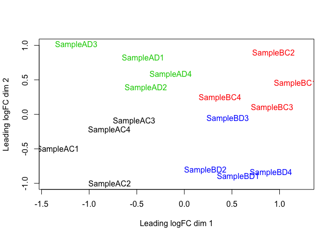
The MDS plot tells you ALOT about what to expect from your experiment.
3. Extracting “normalized” expression table
RPKM vs. FPKM vs. CPM and Model Based
- RPKM - Reads per kilobase per million mapped reads
- FPKM - Fragments per kilobase per million mapped reads
- logCPM – log Counts per million [ good for producing MDS plots, estimate of normalized values in model based ]
- Model based - original read counts are not themselves transformed, but rather correction factors are used in the DE model itself.
We use the cpm function with log=TRUE to approximate normalized expression data.
logcpm <- cpm(d, prior.count=2, log=TRUE)
write.table(logcpm,"rnaseq_workshop_normalized_counts.txt",sep="\t",quote=F)
4. Voom transformation and calculation of variance weights
Specify the model to be fitted. We do this before using voom since voom uses variances of the model residuals (observed - fitted)
mm <- model.matrix(~0 + group)
mm
##    groupA.C groupB.C groupA.D groupB.D
## 1         1        0        0        0
## 2         1        0        0        0
## 3         1        0        0        0
## 4         1        0        0        0
## 5         0        0        1        0
## 6         0        0        1        0
## 7         0        0        1        0
## 8         0        0        1        0
## 9         0        1        0        0
## 10        0        1        0        0
## 11        0        1        0        0
## 12        0        1        0        0
## 13        0        0        0        1
## 14        0        0        0        1
## 15        0        0        0        1
## 16        0        0        0        1
## attr(,"assign")
## [1] 1 1 1 1
## attr(,"contrasts")
## attr(,"contrasts")$group
## [1] "contr.treatment"
The above specifies a model where each coefficient corresponds to a group mean
Voom
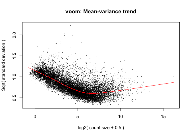
y <- voom(d, mm, plot = T)
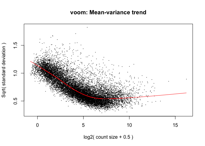
What is voom doing?
- Counts are transformed to log2 counts per million reads (CPM), where “per million reads” is defined based on the normalization factors we calculated earlier
- A linear model is fitted to the log2 CPM for each gene, and the residuals are calculated
- A smoothed curve is fitted to the sqrt(residual standard deviation) by average expression (see red line in plot above)
- The smoothed curve is used to obtain weights for each gene and sample that are passed into limma along with the log2 CPMs.
More details at https://genomebiology.biomedcentral.com/articles/10.1186/gb-2014-15-2-r29
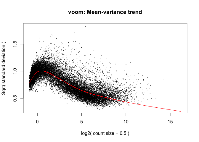
The above is a “good” voom plot. If your voom plot looks like the below, you might want to filter more:
tmp <- voom(d0, mm, plot = T)
Fitting linear models in limma
1. lmFit fits a linear model using weighted least squares for each gene:
fit <- lmFit(y, mm)
head(coef(fit))
##                     groupA.C   groupB.C  groupA.D    groupB.D
## ENSG00000223972.5 -0.5971262 -0.7600101 -2.043466 -0.32633407
## ENSG00000227232.5  2.9541596  2.6168436  2.581553  2.63969481
## ENSG00000238009.6  0.0426848  1.9985563  1.221692 -0.07446036
## ENSG00000268903.1  5.0252475  6.6584763  5.859706  6.22213002
## ENSG00000269981.1  4.7897120  6.3453121  5.534964  6.18975166
## ENSG00000241860.6  1.7040144  3.1693143  3.037286  2.73262246
Comparisons between groups (log fold-changes) are obtained as contrasts of these fitted linear models:
Specify which groups to compare:
Comparison between factor2s C and D for factor1 A
contr <- makeContrasts(groupA.C - groupA.D, levels = colnames(coef(fit)))
contr
##           Contrasts
## Levels     groupA.C - groupA.D
##   groupA.C                   1
##   groupB.C                   0
##   groupA.D                  -1
##   groupB.D                   0
Estimate contrast for each gene
tmp <- contrasts.fit(fit, contr)
The variance characteristics of low expressed genes are different from high expressed genes, if treated the same, the effect is to over represent low expressed genes in the DE list.

Empirical Bayes smoothing of standard errors (shrinks standard errors that are much larger or smaller than those from other genes towards the average standard error) (see https://www.degruyter.com/doi/10.2202/1544-6115.1027)
tmp <- eBayes(tmp)
What genes are most differentially expressed (show the top20)?
top.table <- topTable(tmp, sort.by = "P", n = Inf)
head(top.table, 30)
##                         logFC  AveExpr         t      P.Value   adj.P.Val
## ENSG00000129824.15 -6.0147398 3.826209 -7.151711 7.192005e-07 0.006643531
## ENSG00000067048.16 -6.4034999 2.913309 -6.830168 1.382919e-06 0.006643531
## ENSG00000012817.15 -6.3902747 2.940730 -6.718986 1.739325e-06 0.006643531
## ENSG00000198692.9  -5.1846438 1.887900 -6.693343 1.834216e-06 0.006643531
## ENSG00000099725.14 -5.8261345 2.973758 -6.443233 3.093471e-06 0.008963642
## ENSG00000183878.15 -5.0609574 2.437612 -6.356324 3.716707e-06 0.008974608
## ENSG00000111052.7  -1.6755453 5.558748 -6.134283 5.966643e-06 0.012349247
## ENSG00000114374.12 -5.1961044 1.973817 -5.754669 1.359469e-05 0.022508972
## ENSG00000131002.11 -5.3961967 2.403759 -5.741837 1.398266e-05 0.022508972
## ENSG00000173597.8  -1.3485154 6.533206 -5.420129 2.848455e-05 0.041268410
## ENSG00000131724.10 -1.1406904 7.297997 -5.250323 4.165384e-05 0.054861889
## ENSG00000156052.10 -0.9476761 6.972718 -5.115843 5.639437e-05 0.061469643
## ENSG00000156273.15 -1.1588119 7.548223 -5.100091 5.843804e-05 0.061469643
## ENSG00000112303.13 -1.4642384 9.733935 -5.067169 6.295616e-05 0.061469643
## ENSG00000165178.9  -1.1593005 7.435237 -5.062383 6.364195e-05 0.061469643
## ENSG00000100504.16 -1.2181999 8.577993 -5.011181 7.147213e-05 0.061684964
## ENSG00000257335.8  -1.6909641 7.869467 -5.005615 7.238020e-05 0.061684964
## ENSG00000007237.18 -1.2744658 7.519726 -4.977003 7.723744e-05 0.062167558
## ENSG00000135842.16 -1.3301893 9.052026 -4.937992 8.439855e-05 0.064356114
## ENSG00000116741.7  -1.3080583 8.692475 -4.879201 9.648636e-05 0.068308604
## ENSG00000168461.12 -1.1077995 7.699903 -4.841721 1.050957e-04 0.068308604
## ENSG00000067646.11 -4.1788694 1.091922 -4.825488 1.090626e-04 0.068308604
## ENSG00000177575.12 -1.5598310 5.666019 -4.822239 1.098746e-04 0.068308604
## ENSG00000153317.14 -0.9107735 7.217551 -4.809353 1.131562e-04 0.068308604
## ENSG00000181045.14  1.0410576 4.294615  4.783701 1.199875e-04 0.069535133
## ENSG00000151948.11 -1.2390276 7.449892 -4.746506 1.306421e-04 0.070915945
## ENSG00000101916.11 -1.2155903 7.464792 -4.729317 1.358851e-04 0.070915945
## ENSG00000176597.11 -1.7662280 3.708334 -4.725575 1.370546e-04 0.070915945
## ENSG00000111261.13 -1.4744664 5.657287 -4.627174 1.717464e-04 0.085802135
## ENSG00000105610.5   2.2813253 4.779795  4.574281 1.939395e-04 0.086799278
##                              B
## ENSG00000129824.15  4.68778903
## ENSG00000067048.16  2.96509428
## ENSG00000012817.15  2.97498780
## ENSG00000198692.9   2.13830577
## ENSG00000099725.14  3.05145691
## ENSG00000183878.15  2.50916240
## ENSG00000111052.7   4.01198384
## ENSG00000114374.12  1.50883260
## ENSG00000131002.11  1.84706286
## ENSG00000173597.8   2.62520281
## ENSG00000131724.10  2.27216656
## ENSG00000156052.10  1.98876745
## ENSG00000156273.15  1.95560743
## ENSG00000112303.13  1.88678950
## ENSG00000165178.9   1.87570274
## ENSG00000100504.16  1.76807027
## ENSG00000257335.8   1.75585054
## ENSG00000007237.18  1.69460425
## ENSG00000135842.16  1.61410567
## ENSG00000116741.7   1.48853574
## ENSG00000168461.12  1.40598506
## ENSG00000067646.11 -0.05126028
## ENSG00000177575.12  1.37070688
## ENSG00000153317.14  1.33627398
## ENSG00000181045.14  1.28704220
## ENSG00000151948.11  1.20219270
## ENSG00000101916.11  1.16527497
## ENSG00000176597.11  0.99700634
## ENSG00000111261.13  0.95969143
## ENSG00000105610.5   0.78163768
- logFC: log2 fold change of A.C/A.D
- AveExpr: Average expression across all samples, in log2 CPM
- t: logFC divided by its standard error
- P.Value: Raw p-value (based on t) from test that logFC differs from 0
- adj.P.Val: Benjamini-Hochberg false discovery rate adjusted p-value
- B: log-odds that gene is DE (arguably less useful than the other columns)
ENSG00000129824.15 has higher expression at factor2 D than at factor2 C (logFC is netative). ENSG00000181045.14 has higher expression at factor2 C than at factor2 D (logFC is positive).
How many DE genes are there?
length(which(top.table$adj.P.Val < 0.05))
## [1] 10
Multiple Testing Correction
- Simply a must! Best choices are:
- FDR (false discovery rate), such as BH.
- Qvalue
-
The FDR (or qvalue) is a statement about the list and is no longer about the gene (pvalue). So a FDR of 0.05, says you expect 5% false positives in the list of genes with an FDR of 0.05 or less.
- The statement “Statistically significant” means FDR of 0.05 or less. My opinion is these genes do not require further validation (e.g. with qrtPCR) You can dip below the FDR of 0.05, but in my opinion you then need to validate those genes (e.g. with qrtPCR)
Write top.table to a file, adding in cpms and annotation
top.table$Gene <- rownames(top.table)
top.table <- top.table[,c("Gene", names(top.table)[1:6])]

top.table <- data.frame(top.table,anno[match(top.table$Gene,anno$Gene.stable.ID.version),],logcpm[match(top.table$Gene,rownames(logcpm)),])

write.table(top.table, file = "A.C_v_A.D.txt", row.names = F, sep = "\t", quote = F)
Let’s say we want to compare factor1s A and B at factor2 C. The only thing we have to change is the call to makeContrasts:
contr <- makeContrasts(groupA.C - groupB.C, levels = colnames(coef(fit)))
tmp <- contrasts.fit(fit, contr)
tmp <- eBayes(tmp)
top.table <- topTable(tmp, sort.by = "P", n = Inf)
head(top.table, 20)
##                        logFC  AveExpr         t      P.Value    adj.P.Val
## ENSG00000100504.16 -2.376956 8.577993 -9.704544 6.496525e-09 9.412165e-05
## ENSG00000257335.8  -3.157310 7.869467 -9.239181 1.440800e-08 1.043716e-04
## ENSG00000115828.16 -2.329031 6.982374 -8.914077 2.552955e-08 1.155460e-04
## ENSG00000111261.13 -2.736523 5.657287 -8.649484 4.106524e-08 1.155460e-04
## ENSG00000135636.13 -2.810823 8.693319 -8.603541 4.463872e-08 1.155460e-04
## ENSG00000153317.14 -1.550277 7.217551 -8.199242 9.412370e-08 1.155460e-04
## ENSG00000151948.11 -2.139321 7.449892 -8.184490 9.675982e-08 1.155460e-04
## ENSG00000184678.10 -1.962494 5.446002 -8.181176 9.736252e-08 1.155460e-04
## ENSG00000106780.8  -1.757438 8.586755 -8.174915 9.851183e-08 1.155460e-04
## ENSG00000136040.8  -1.937641 8.641023 -8.122811 1.086394e-07 1.155460e-04
## ENSG00000151726.13 -2.619849 9.882600 -8.122380 1.087276e-07 1.155460e-04
## ENSG00000140563.14 -1.887358 6.641187 -8.110484 1.111898e-07 1.155460e-04
## ENSG00000115590.13 -2.933426 6.040275 -8.078369 1.181300e-07 1.155460e-04
## ENSG00000173597.8  -2.000869 6.533206 -8.048820 1.249127e-07 1.155460e-04
## ENSG00000062282.14 -2.280380 7.536446 -8.019791 1.319700e-07 1.155460e-04
## ENSG00000111052.7  -2.194636 5.558748 -8.010015 1.344386e-07 1.155460e-04
## ENSG00000196663.15 -2.170473 6.832034 -7.975266 1.436079e-07 1.155460e-04
## ENSG00000146094.14 -1.979674 8.645284 -7.940617 1.533981e-07 1.155460e-04
## ENSG00000059804.15 -2.107665 8.534423 -7.897353 1.666021e-07 1.155460e-04
## ENSG00000103569.9  -2.348441 9.716634 -7.896060 1.670143e-07 1.155460e-04
##                            B
## ENSG00000100504.16 10.615370
## ENSG00000257335.8   9.868599
## ENSG00000115828.16  9.330894
## ENSG00000111261.13  8.806668
## ENSG00000135636.13  8.794859
## ENSG00000153317.14  8.092020
## ENSG00000151948.11  8.064204
## ENSG00000184678.10  8.015052
## ENSG00000106780.8   8.043185
## ENSG00000136040.8   7.949306
## ENSG00000151726.13  7.935342
## ENSG00000140563.14  7.929025
## ENSG00000115590.13  7.837023
## ENSG00000173597.8   7.815062
## ENSG00000062282.14  7.766186
## ENSG00000111052.7   7.703886
## ENSG00000196663.15  7.683394
## ENSG00000146094.14  7.618792
## ENSG00000059804.15  7.539748
## ENSG00000103569.9   7.529803
length(which(top.table$adj.P.Val < 0.05)) # number of DE genes
## [1] 3267
top.table$Gene <- rownames(top.table)
top.table <- top.table[,c("Gene", names(top.table)[1:6])]

top.table <- data.frame(top.table,anno[match(top.table$Gene,anno$Gene.stable.ID.version),],logcpm[match(top.table$Gene,rownames(logcpm)),])

write.table(top.table, file = "A.C_v_B.C.txt", row.names = F, sep = "\t", quote = F)
What if we refit our model as a two-factor model (rather than using the group variable)?
Create new model matrix:
mm <- model.matrix(~factor1*factor2)
mm
##    (Intercept) factor1B factor2D factor1B:factor2D
## 1            1        0        0                 0
## 2            1        0        0                 0
## 3            1        0        0                 0
## 4            1        0        0                 0
## 5            1        0        1                 0
## 6            1        0        1                 0
## 7            1        0        1                 0
## 8            1        0        1                 0
## 9            1        1        0                 0
## 10           1        1        0                 0
## 11           1        1        0                 0
## 12           1        1        0                 0
## 13           1        1        1                 1
## 14           1        1        1                 1
## 15           1        1        1                 1
## 16           1        1        1                 1
## attr(,"assign")
## [1] 0 1 2 3
## attr(,"contrasts")
## attr(,"contrasts")$factor1
## [1] "contr.treatment"
##
## attr(,"contrasts")$factor2
## [1] "contr.treatment"
We are specifying that model includes effects for factor1, factor2, and the factor1-factor2 interaction (which allows the differences between factor1s to differ across factor2)
colnames(mm)
## [1] "(Intercept)"       "factor1B"          "factor2D"
## [4] "factor1B:factor2D"
y <- voom(d, mm, plot = F)
fit <- lmFit(y, mm)
head(coef(fit))
##                   (Intercept)   factor1B   factor2D factor1B:factor2D
## ENSG00000223972.5  -0.5971262 -0.1628838 -1.4463397         1.8800157
## ENSG00000227232.5   2.9541596 -0.3373160 -0.3726064         0.3954576
## ENSG00000238009.6   0.0426848  1.9558715  1.1790068        -3.2520235
## ENSG00000268903.1   5.0252475  1.6332288  0.8344581        -1.2708044
## ENSG00000269981.1   4.7897120  1.5556001  0.7452518        -0.9008122
## ENSG00000241860.6   1.7040144  1.4652998  1.3332714        -1.7699632
- The coefficient factor1B represents the difference in mean expression between factor1 B and the reference factor1 (factor1 A), for factor2 C (the reference level for factor2)
- The coefficient factor2D represents the difference in mean expression between factor2 D and factor2 C, for factor1 A
- The coefficient factor1B:factor2D is the difference between factor2s D and C of the differences between factor1s B and A (the interaction effect)
Let’s estimate the difference between factor1s A and B at factor2 C
tmp <- contrasts.fit(fit, coef = 2) # Directly test second coefficient
tmp <- eBayes(tmp)
top.table <- topTable(tmp, sort.by = "P", n = Inf)
head(top.table, 20)
##                       logFC  AveExpr        t      P.Value    adj.P.Val
## ENSG00000100504.16 2.376956 8.577993 9.704544 6.496525e-09 9.412165e-05
## ENSG00000257335.8  3.157310 7.869467 9.239181 1.440800e-08 1.043716e-04
## ENSG00000115828.16 2.329031 6.982374 8.914077 2.552955e-08 1.155460e-04
## ENSG00000111261.13 2.736523 5.657287 8.649484 4.106524e-08 1.155460e-04
## ENSG00000135636.13 2.810823 8.693319 8.603541 4.463872e-08 1.155460e-04
## ENSG00000153317.14 1.550277 7.217551 8.199242 9.412370e-08 1.155460e-04
## ENSG00000151948.11 2.139321 7.449892 8.184490 9.675982e-08 1.155460e-04
## ENSG00000184678.10 1.962494 5.446002 8.181176 9.736252e-08 1.155460e-04
## ENSG00000106780.8  1.757438 8.586755 8.174915 9.851183e-08 1.155460e-04
## ENSG00000136040.8  1.937641 8.641023 8.122811 1.086394e-07 1.155460e-04
## ENSG00000151726.13 2.619849 9.882600 8.122380 1.087276e-07 1.155460e-04
## ENSG00000140563.14 1.887358 6.641187 8.110484 1.111898e-07 1.155460e-04
## ENSG00000115590.13 2.933426 6.040275 8.078369 1.181300e-07 1.155460e-04
## ENSG00000173597.8  2.000869 6.533206 8.048820 1.249127e-07 1.155460e-04
## ENSG00000062282.14 2.280380 7.536446 8.019791 1.319700e-07 1.155460e-04
## ENSG00000111052.7  2.194636 5.558748 8.010015 1.344386e-07 1.155460e-04
## ENSG00000196663.15 2.170473 6.832034 7.975266 1.436079e-07 1.155460e-04
## ENSG00000146094.14 1.979674 8.645284 7.940617 1.533981e-07 1.155460e-04
## ENSG00000059804.15 2.107665 8.534423 7.897353 1.666021e-07 1.155460e-04
## ENSG00000103569.9  2.348441 9.716634 7.896060 1.670143e-07 1.155460e-04
##                            B
## ENSG00000100504.16 10.615370
## ENSG00000257335.8   9.868599
## ENSG00000115828.16  9.330894
## ENSG00000111261.13  8.806668
## ENSG00000135636.13  8.794859
## ENSG00000153317.14  8.092020
## ENSG00000151948.11  8.064204
## ENSG00000184678.10  8.015052
## ENSG00000106780.8   8.043185
## ENSG00000136040.8   7.949306
## ENSG00000151726.13  7.935342
## ENSG00000140563.14  7.929025
## ENSG00000115590.13  7.837023
## ENSG00000173597.8   7.815062
## ENSG00000062282.14  7.766186
## ENSG00000111052.7   7.703886
## ENSG00000196663.15  7.683394
## ENSG00000146094.14  7.618792
## ENSG00000059804.15  7.539748
## ENSG00000103569.9   7.529803
length(which(top.table$adj.P.Val < 0.05)) # number of DE genes
## [1] 3267
We get the same results as with the model where each coefficient corresponded to a group mean. In essence, these are the same model, so use whichever is most convenient for what you are estimating.
The interaction effects factor1B:factor2D are easier to estimate and test in this setup
head(coef(fit))
##                   (Intercept)   factor1B   factor2D factor1B:factor2D
## ENSG00000223972.5  -0.5971262 -0.1628838 -1.4463397         1.8800157
## ENSG00000227232.5   2.9541596 -0.3373160 -0.3726064         0.3954576
## ENSG00000238009.6   0.0426848  1.9558715  1.1790068        -3.2520235
## ENSG00000268903.1   5.0252475  1.6332288  0.8344581        -1.2708044
## ENSG00000269981.1   4.7897120  1.5556001  0.7452518        -0.9008122
## ENSG00000241860.6   1.7040144  1.4652998  1.3332714        -1.7699632
tmp <- contrasts.fit(fit, coef = 4) # Test factor1B:factor2D
tmp <- eBayes(tmp)
top.table <- topTable(tmp, sort.by = "P", n = Inf)
head(top.table, 20)
##                         logFC  AveExpr         t      P.Value    adj.P.Val
## ENSG00000198692.9  -11.314189 1.887900 -9.485646 9.418828e-09 0.0001364600
## ENSG00000067048.16 -13.225631 2.913309 -8.627328 4.274986e-08 0.0002373427
## ENSG00000012817.15 -13.827790 2.940730 -8.542373 4.990445e-08 0.0002373427
## ENSG00000183878.15 -11.123998 2.437612 -8.394064 6.552808e-08 0.0002373427
## ENSG00000129824.15 -13.034887 3.826209 -7.922001 1.589416e-07 0.0004605491
## ENSG00000099725.14 -12.293405 2.973758 -7.605966 2.924361e-07 0.0007061357
## ENSG00000114374.12 -10.697056 1.973817 -7.206407 6.443949e-07 0.0013337132
## ENSG00000131002.11 -11.419184 2.403759 -6.954224 1.072828e-06 0.0018129284
## ENSG00000111052.7   -2.572035 5.558748 -6.930424 1.126198e-06 0.0018129284
## ENSG00000100485.11  -1.560909 6.534916 -6.834468 1.370754e-06 0.0019859480
## ENSG00000173597.8   -2.261255 6.533206 -6.515146 2.659575e-06 0.0035029026
## ENSG00000119669.4   -1.531074 6.231767 -6.160246 5.643536e-06 0.0068136296
## ENSG00000140563.14  -1.971119 6.641187 -6.038877 7.326430e-06 0.0077335313
## ENSG00000111261.13  -2.560364 5.657287 -6.029697 7.473042e-06 0.0077335313
## ENSG00000135049.15  -1.626519 6.700731 -5.881437 1.030613e-05 0.0093485695
## ENSG00000067646.11  -7.996768 1.091922 -5.851877 1.099175e-05 0.0093485695
## ENSG00000143622.10  -1.444739 5.881461 -5.833176 1.144952e-05 0.0093485695
## ENSG00000257335.8   -2.797746 7.869467 -5.826613 1.161473e-05 0.0093485695
## ENSG00000151948.11  -2.115808 7.449892 -5.738633 1.408129e-05 0.0107373516
## ENSG00000178904.18  -1.912908 4.651897 -5.663440 1.661233e-05 0.0120339684
##                           B
## ENSG00000198692.9  5.297834
## ENSG00000067048.16 5.162789
## ENSG00000012817.15 5.025682
## ENSG00000183878.15 4.976220
## ENSG00000129824.15 5.220342
## ENSG00000099725.14 4.393210
## ENSG00000114374.12 3.494078
## ENSG00000131002.11 3.411359
## ENSG00000111052.7  5.674172
## ENSG00000100485.11 5.509396
## ENSG00000173597.8  4.876389
## ENSG00000119669.4  4.157010
## ENSG00000140563.14 3.905815
## ENSG00000111261.13 3.891350
## ENSG00000135049.15 3.577235
## ENSG00000067646.11 1.608406
## ENSG00000143622.10 3.482269
## ENSG00000257335.8  3.464937
## ENSG00000151948.11 3.277440
## ENSG00000178904.18 3.125817
length(which(top.table$adj.P.Val < 0.05))
## [1] 242
The log fold change here is the difference between factor1 B and factor1 A in the log fold changes between factor2s D and C.
A gene for which this interaction effect is significant is one for which the effect of factor2 differs between factor1s, and for which the effect of factor1 differs between factor2s.
2. More complicated models Specifying a different model is simply a matter of changing the calls to model.matrix (and possibly to contrasts.fit).
Let’s say we have information on the RNA extraction batch:
batch <- factor(rep(rep(1:2, each = 2), 4))
batch
##  [1] 1 1 2 2 1 1 2 2 1 1 2 2 1 1 2 2
## Levels: 1 2
To adjust for batch in the analysis, add batch to the end of the call to model matrix. Everything else about the code stays the same:
mm <- model.matrix(~0 + group + batch)
mm
##    groupA.C groupB.C groupA.D groupB.D batch2
## 1         1        0        0        0      0
## 2         1        0        0        0      0
## 3         1        0        0        0      1
## 4         1        0        0        0      1
## 5         0        0        1        0      0
## 6         0        0        1        0      0
## 7         0        0        1        0      1
## 8         0        0        1        0      1
## 9         0        1        0        0      0
## 10        0        1        0        0      0
## 11        0        1        0        0      1
## 12        0        1        0        0      1
## 13        0        0        0        1      0
## 14        0        0        0        1      0
## 15        0        0        0        1      1
## 16        0        0        0        1      1
## attr(,"assign")
## [1] 1 1 1 1 2
## attr(,"contrasts")
## attr(,"contrasts")$group
## [1] "contr.treatment"
##
## attr(,"contrasts")$batch
## [1] "contr.treatment"
y <- voom(d, mm, plot = F)
fit <- lmFit(y, mm)
contr <- makeContrasts(groupB.D - groupA.D, levels = colnames(coef(fit)))
tmp <- contrasts.fit(fit, contr)
tmp <- eBayes(tmp)
top.table <- topTable(tmp, sort.by = "P", n = Inf)
head(top.table, 20)
##                         logFC    AveExpr         t      P.Value  adj.P.Val
## ENSG00000260231.2   1.9908670  4.3090858  7.153855 9.740906e-07 0.01400593
## ENSG00000105610.5   3.2699187  4.7797951  6.803931 1.933452e-06 0.01400593
## ENSG00000198692.9  -5.6713490  1.8879002 -6.345696 4.864867e-06 0.02141957
## ENSG00000206177.6   3.5470364  5.5073482  6.023185 9.470037e-06 0.02141957
## ENSG00000067048.16 -7.1997748  2.9133089 -5.933366 1.142753e-05 0.02141957
## ENSG00000164068.15  1.7096353  6.4547630  5.786748 1.556319e-05 0.02141957
## ENSG00000070614.14  1.4214439  6.4301848  5.768240 1.618508e-05 0.02141957
## ENSG00000104903.4   1.5367805  7.6102639  5.722040 1.785124e-05 0.02141957
## ENSG00000260592.1   2.5605829  4.4181706  5.708117 1.838719e-05 0.02141957
## ENSG00000012817.15 -7.6626834  2.9407300 -5.697772 1.879604e-05 0.02141957
## ENSG00000142784.15  0.9444748  7.7901380  5.685762 1.928247e-05 0.02141957
## ENSG00000184481.16  1.5014451  7.0621560  5.630289 2.170256e-05 0.02141957
## ENSG00000174358.15  3.7662019 -0.1572361  5.611026 2.261408e-05 0.02141957
## ENSG00000132819.16  2.4549059  9.1890963  5.577215 2.431012e-05 0.02141957
## ENSG00000167992.12  3.2891276  3.9854034  5.576935 2.432466e-05 0.02141957
## ENSG00000008441.16  2.5527445  5.9254779  5.550620 2.573547e-05 0.02141957
## ENSG00000134779.14  1.8635011  6.3278733  5.504039 2.844198e-05 0.02141957
## ENSG00000170271.10  2.7459963  5.9409165  5.481593 2.984867e-05 0.02141957
## ENSG00000183878.15 -5.8835494  2.4376117 -5.460263 3.125151e-05 0.02141957
## ENSG00000090674.15  1.6399830  5.5303379  5.444477 3.233311e-05 0.02141957
##                           B
## ENSG00000260231.2  5.769473
## ENSG00000105610.5  5.101320
## ENSG00000198692.9  2.481087
## ENSG00000206177.6  3.688778
## ENSG00000067048.16 2.122112
## ENSG00000164068.15 3.178022
## ENSG00000070614.14 3.137366
## ENSG00000104903.4  3.041415
## ENSG00000260592.1  3.043986
## ENSG00000012817.15 1.731381
## ENSG00000142784.15 2.967565
## ENSG00000184481.16 2.849133
## ENSG00000174358.15 1.038449
## ENSG00000132819.16 2.756914
## ENSG00000167992.12 2.752915
## ENSG00000008441.16 2.715297
## ENSG00000134779.14 2.593540
## ENSG00000170271.10 2.571686
## ENSG00000183878.15 1.456446
## ENSG00000090674.15 2.488309
length(which(top.table$adj.P.Val < 0.05))
## [1] 189
What if we want to adjust for a continuous variable like RIN score:
# Generate example RIN data
set.seed(99)
RIN <- rnorm(n = 16, mean = 7.5, sd = 1)
RIN
##  [1] 7.713963 7.979658 7.587829 7.943859 7.137162 7.622674 6.636155
##  [8] 7.989624 7.135883 6.205758 6.754231 8.421550 8.250054 4.991446
## [15] 4.459066 7.500266
Model adjusting for RIN score
mm <- model.matrix(~0 + group + RIN)
y <- voom(d, mm, plot = F)
fit <- lmFit(y, mm)
contr <- makeContrasts(groupB.D - groupA.D, levels = colnames(coef(fit)))
tmp <- contrasts.fit(fit, contr)
tmp <- eBayes(tmp)
top.table <- topTable(tmp, sort.by = "P", n = Inf)
head(top.table, 20)
##                        logFC    AveExpr          t      P.Value
## ENSG00000198692.9  -6.006955  1.8879002 -10.866375 1.732871e-09
## ENSG00000067048.16 -7.300716  2.9133089  -9.959856 6.976176e-09
## ENSG00000012817.15 -7.758516  2.9407300  -9.873085 8.008435e-09
## ENSG00000129824.15 -7.735443  3.8262088  -8.855309 4.313678e-08
## ENSG00000183878.15 -5.734474  2.4376117  -8.420362 9.205807e-08
## ENSG00000099725.14 -6.786515  2.9737584  -8.137237 1.527532e-07
## ENSG00000114374.12 -6.344711  1.9738173  -8.017824 1.897167e-07
## ENSG00000105610.5   3.330123  4.7797951   7.995327 1.976640e-07
## ENSG00000131002.11 -6.859349  2.4037588  -7.949944 2.147667e-07
## ENSG00000167992.12  3.481323  3.9854034   7.554362 4.478539e-07
## ENSG00000017483.14  2.728747  5.9726590   7.539403 4.606631e-07
## ENSG00000260231.2   1.990333  4.3090858   7.462830 5.324536e-07
## ENSG00000187244.11  5.599997  1.8991871   7.365141 6.412439e-07
## ENSG00000174358.15  4.000132 -0.1572361   7.101164 1.066608e-06
## ENSG00000145423.4   4.803616  1.0290221   7.045901 1.187916e-06
## ENSG00000205639.10  3.273983  3.6022475   6.929916 1.491257e-06
## ENSG00000260592.1   2.755993  4.4181706   6.844285 1.765957e-06
## ENSG00000213088.10  4.112311  1.5380190   6.698291 2.361347e-06
## ENSG00000164068.15  1.901266  6.4547630   6.614858 2.791448e-06
## ENSG00000102145.13  2.511509  5.0898109   6.610723 2.814767e-06
##                       adj.P.Val        B
## ENSG00000198692.9  2.510584e-05 9.808124
## ENSG00000067048.16 3.867540e-05 9.340123
## ENSG00000012817.15 3.867540e-05 9.175836
## ENSG00000129824.15 1.562414e-04 8.080075
## ENSG00000183878.15 2.667475e-04 7.195578
## ENSG00000099725.14 3.457267e-04 6.894271
## ENSG00000114374.12 3.457267e-04 6.345491
## ENSG00000105610.5  3.457267e-04 7.371076
## ENSG00000131002.11 3.457267e-04 6.449662
## ENSG00000167992.12 6.067352e-04 6.569346
## ENSG00000017483.14 6.067352e-04 6.588291
## ENSG00000260231.2  6.428490e-04 6.417935
## ENSG00000187244.11 7.146417e-04 5.383435
## ENSG00000174358.15 1.103787e-03 3.888410
## ENSG00000145423.4  1.147368e-03 4.459281
## ENSG00000205639.10 1.350334e-03 5.397929
## ENSG00000260592.1  1.505011e-03 5.285921
## ENSG00000213088.10 1.900622e-03 4.284445
## ENSG00000164068.15 2.039017e-03 4.834114
## ENSG00000102145.13 2.039017e-03 4.841848
length(which(top.table$adj.P.Val < 0.05))
## [1] 456
What if we want to look at the correlation of gene expression with a continuous variable like pH?
# Generate example pH data
set.seed(99)
pH <- rnorm(n = 16, mean = 8, sd = 1.5)
pH
##  [1] 8.320944 8.719487 8.131743 8.665788 7.455743 8.184011 6.704232
##  [8] 8.734436 7.453825 6.058637 6.881346 9.382326 9.125082 4.237169
## [15] 3.438599 8.000399
Specify model matrix:
mm <- model.matrix(~pH)
head(mm)
##   (Intercept)       pH
## 1           1 8.320944
## 2           1 8.719487
## 3           1 8.131743
## 4           1 8.665788
## 5           1 7.455743
## 6           1 8.184011
y <- voom(d, mm, plot = F)
fit <- lmFit(y, mm)
tmp <- contrasts.fit(fit, coef = 2) # test "pH" coefficient
tmp <- eBayes(tmp)
top.table <- topTable(tmp, sort.by = "P", n = Inf)
head(top.table, 20)
##                         logFC    AveExpr         t      P.Value adj.P.Val
## ENSG00000265992.1  -1.1267300  0.4043486 -6.015318 6.912725e-06 0.1001516
## ENSG00000099864.17 -0.5935954 -0.2070152 -4.831938 1.004230e-04 0.4610971
## ENSG00000230910.3  -0.5954909  0.2372561 -4.730234 1.271254e-04 0.4610971
## ENSG00000273855.1  -0.3959891  0.9398840 -4.643645 1.554639e-04 0.4610971
## ENSG00000168386.18 -0.5257880 -0.5419708 -4.338886 3.165661e-04 0.4610971
## ENSG00000085871.8  -0.3419470  3.6234894 -4.324451 3.274371e-04 0.4610971
## ENSG00000281404.1  -0.3748794  1.2402290 -4.318328 3.321611e-04 0.4610971
## ENSG00000115919.14 -0.2861967  4.4939851 -4.313879 3.356365e-04 0.4610971
## ENSG00000237541.3  -0.6540314  2.3156583 -4.308179 3.401423e-04 0.4610971
## ENSG00000175866.15 -0.3272373  2.9101111 -4.274589 3.679564e-04 0.4610971
## ENSG00000172322.13 -0.5575537  6.7723566 -4.234522 4.041345e-04 0.4610971
## ENSG00000147804.9  -0.3142993  1.9875624 -4.213326 4.246944e-04 0.4610971
## ENSG00000197632.8  -0.4562314  1.0442273 -4.205147 4.329059e-04 0.4610971
## ENSG00000136205.16 -0.2470392  4.6482208 -4.189429 4.491352e-04 0.4610971
## ENSG00000104918.7  -0.6636665  2.7085179 -4.163374 4.773921e-04 0.4610971
## ENSG00000242498.7  -0.3270991  3.8774772 -4.113718 5.362653e-04 0.4855883
## ENSG00000211749.1   0.5638714  0.6057260  3.998422 7.024939e-04 0.5645317
## ENSG00000186049.8   0.6149507  1.6900224  3.988341 7.192716e-04 0.5645317
## ENSG00000008277.14  0.6550436  1.2861630  3.976008 7.403438e-04 0.5645317
## ENSG00000166436.16  0.2714735  4.8549612  3.906884 8.703514e-04 0.6083973
##                              B
## ENSG00000265992.1   0.75227001
## ENSG00000099864.17 -1.39564889
## ENSG00000230910.3  -1.06062381
## ENSG00000273855.1  -1.01341997
## ENSG00000168386.18 -2.05522385
## ENSG00000085871.8  -0.04835452
## ENSG00000281404.1  -1.19086186
## ENSG00000115919.14  0.12244786
## ENSG00000237541.3  -0.38850331
## ENSG00000175866.15 -0.41097644
## ENSG00000172322.13 -0.02164101
## ENSG00000147804.9  -0.94156968
## ENSG00000197632.8  -1.29233557
## ENSG00000136205.16 -0.09513872
## ENSG00000104918.7  -0.46363997
## ENSG00000242498.7  -0.33718514
## ENSG00000211749.1  -2.68448251
## ENSG00000186049.8  -2.28398324
## ENSG00000008277.14 -2.50098587
## ENSG00000166436.16 -0.75038804
length(which(top.table$adj.P.Val < 0.05))
## [1] 0
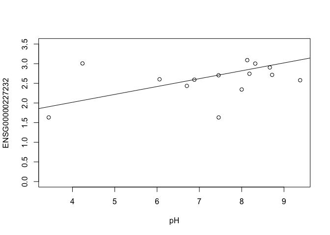
In this case, limma is fitting a linear regression model, which here is a straight line fit, with the slope and intercept defined by the model coefficients:
ENSG00000227232 <- y$E["ENSG00000227232.5",]
plot(ENSG00000227232 ~ pH, ylim = c(0, 3.5))
intercept <- coef(fit)["ENSG00000227232.5", "(Intercept)"]
slope <- coef(fit)["ENSG00000227232.5", "pH"]
abline(a = intercept, b = slope)
slope
## [1] 0.2004075
In this example, the log fold change logFC is the slope of the line, or the change in gene expression (on the log2 CPM scale) for each unit increase in pH.
Here, a logFC of 0.20 means a 0.20 log2 CPM increase in gene expression for each unit increase in pH, or a 15% increase on the CPM scale (2^0.20 = 1.15).
3. A bit more on linear models
Limma fits a linear model to each gene.
Linear models include analysis of variance (ANOVA) models, linear regression, and any model of the form
The covariates X can be:
- a continuous variable (pH, RIN score, age, weight, temperature, etc.)
- Dummy variables coding a categorical covariate (like factor1, factor2, and group)
The $\beta$’s are unknown parameters to be estimated.
In limma, the $\beta$’s are the log fold changes.
The error (residual) term $\epsilon$ is assumed to be normally distributed with a variance that is constant across the range of the data.
Normally distributed means the residuals come from a distribution that looks like this:
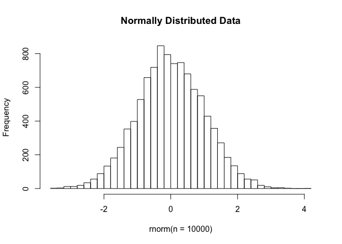
The log2 transformation that voom applies to the counts makes the data “normal enough”, but doesn’t completely stabilize the variance:
tmp <- voom(d, mm, plot = T)
The log2 counts per million are more variable at lower expression levels. The variance weights calculated by voom address this situation.
Simple plotting
mm <- model.matrix(~factor1*factor2)
colnames(mm) <- make.names(colnames(mm))
y <- voom(d, mm, plot = F)
fit <- lmFit(y, mm)

contrast.matrix <- makeContrasts(factor1B, factor2D, levels=colnames(coef(fit)))
fit2 <- contrasts.fit(fit, contrast.matrix)
fit2 <- eBayes(fit2)
top.table <- topTable(fit2, coef = 1, sort.by = "P", n = 40)
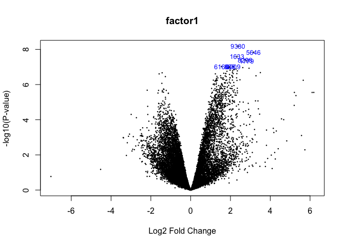
1. Volcano plot
volcanoplot(fit2,coef=1,highlight=8,names=fit$genes$NAME,main="factor1")
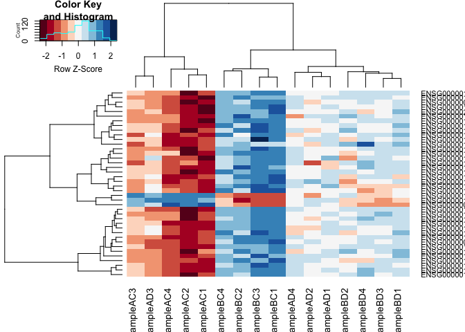
2. Heatmap
#using a red and blue colour scheme without traces and scaling each row
heatmap.2(logcpm[rownames(top.table),],col=brewer.pal(11,"RdBu"),scale="row", trace="none")
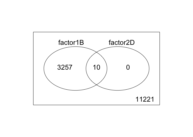
3. 2 factor venn diagram
results <- decideTests(fit2)
vennDiagram(results)
Both edgeR and limma voom have VERY comprehensive user manuals
sessionInfo()
## R version 3.5.2 (2018-12-20)
## Platform: x86_64-apple-darwin15.6.0 (64-bit)
## Running under: macOS Mojave 10.14.3
##
## Matrix products: default
## BLAS: /Library/Frameworks/R.framework/Versions/3.5/Resources/lib/libRblas.0.dylib
## LAPACK: /Library/Frameworks/R.framework/Versions/3.5/Resources/lib/libRlapack.dylib
##
## locale:
## [1] en_US.UTF-8/en_US.UTF-8/en_US.UTF-8/C/en_US.UTF-8/en_US.UTF-8
##
## attached base packages:
## [1] stats     graphics  grDevices utils     datasets  methods   base
##
## other attached packages:
## [1] gplots_3.0.1       RColorBrewer_1.1-2 edgeR_3.24.3
## [4] limma_3.38.3
##
## loaded via a namespace (and not attached):
##  [1] locfit_1.5-9.1     Rcpp_1.0.0         lattice_0.20-38
##  [4] gtools_3.8.1       digest_0.6.18      bitops_1.0-6
##  [7] grid_3.5.2         magrittr_1.5       evaluate_0.12
## [10] KernSmooth_2.23-15 stringi_1.2.4      gdata_2.18.0
## [13] rmarkdown_1.11     tools_3.5.2        stringr_1.3.1
## [16] xfun_0.4           yaml_2.2.0         compiler_3.5.2
## [19] caTools_1.17.1.1   htmltools_0.3.6    knitr_1.21