
Introduction to Single Cell RNA-Seq Part 6: Clustering and cell type assignment
Clustering and cell type assignment are critical steps in many single cell (or single nucleus) experiments. The power of single cell experiments is to capture the heterogeneity within samples as well as between them. Clustering permits the user to organize cells into clusters that correspond to biologically and experimentally relevant populations.
Set up workspace
library(Seurat)
library(kableExtra)
library(tidyr)
library(dplyr)
library(ggplot2)
library(HGNChelper)
library(ComplexHeatmap)
set.seed(12345)
experiment.aggregate <- readRDS("scRNA_workshop-04.rds")
experiment.aggregate
## An object of class Seurat
## 11474 features across 6315 samples within 1 assay
## Active assay: RNA (11474 features, 7110 variable features)
##  3 layers present: counts, data, scale.data
##  2 dimensional reductions calculated: pca, umap
Construct network
Seurat implements an graph-based clustering approach. Distances between the cells are calculated based on previously identified PCs.
The default method for identifying k-nearest neighbors is annoy, an approximate nearest-neighbor approach that is widely used for high-dimensional analysis in many fields, including single-cell analysis. Extensive community benchmarking has shown that annoy substantially improves the speed and memory requirements of neighbor discovery, with negligible impact to downstream results.
experiment.aggregate <- FindNeighbors(experiment.aggregate, reduction = "pca", dims = 1:50)
Find clusters
The FindClusters function implements the neighbor based clustering procedure, and contains a resolution parameter that sets the granularity of the downstream clustering, with increased values leading to a greater number of clusters. This code produces a series of resolutions for us to investigate and choose from.
The clustering resolution parameter is unit-less and somewhat arbitrary. The resolutions used here were selected to produce a useable number of clusters in the example experiment.
experiment.aggregate <- FindClusters(experiment.aggregate,
                                     resolution = seq(0.1, 0.4, 0.1))
## Modularity Optimizer version 1.3.0 by Ludo Waltman and Nees Jan van Eck
##
## Number of nodes: 6315
## Number of edges: 259289
##
## Running Louvain algorithm...
## Maximum modularity in 10 random starts: 0.9690
## Number of communities: 10
## Elapsed time: 0 seconds
## Modularity Optimizer version 1.3.0 by Ludo Waltman and Nees Jan van Eck
##
## Number of nodes: 6315
## Number of edges: 259289
##
## Running Louvain algorithm...
## Maximum modularity in 10 random starts: 0.9494
## Number of communities: 11
## Elapsed time: 0 seconds
## Modularity Optimizer version 1.3.0 by Ludo Waltman and Nees Jan van Eck
##
## Number of nodes: 6315
## Number of edges: 259289
##
## Running Louvain algorithm...
## Maximum modularity in 10 random starts: 0.9343
## Number of communities: 14
## Elapsed time: 0 seconds
## Modularity Optimizer version 1.3.0 by Ludo Waltman and Nees Jan van Eck
##
## Number of nodes: 6315
## Number of edges: 259289
##
## Running Louvain algorithm...
## Maximum modularity in 10 random starts: 0.9224
## Number of communities: 17
## Elapsed time: 0 seconds
Seurat adds the clustering information to the metadata table. Each FindClusters call generates a new column named with the assay, followed by “_snn_res.”, and the resolution.
cluster.resolutions <- grep("res", colnames(experiment.aggregate@meta.data), value = TRUE)
head(experiment.aggregate@meta.data[,cluster.resolutions]) %>%
  kable(caption = 'Cluster identities are added to the meta.data slot.') %>%
  kable_styling("striped")
| RNA_snn_res.0.1 | RNA_snn_res.0.2 | RNA_snn_res.0.3 | RNA_snn_res.0.4 | |
|---|---|---|---|---|
| AAACCCAAGTTATGGA_A001-C-007 | 1 | 1 | 2 | 10 |
| AAACGCTTCTCTGCTG_A001-C-007 | 6 | 7 | 9 | 13 |
| AAAGAACGTGCTTATG_A001-C-007 | 1 | 1 | 4 | 5 |
| AAAGAACGTTTCGCTC_A001-C-007 | 3 | 3 | 3 | 3 |
| AAAGAACTCTGGCTGG_A001-C-007 | 4 | 5 | 7 | 8 |
| AAAGGATTCATTACCT_A001-C-007 | 3 | 3 | 3 | 3 |
Explore clustering resolutions
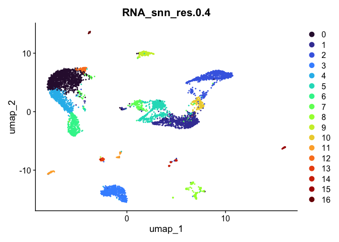
The number of clusters produced increases with the clustering resolution.
sapply(cluster.resolutions, function(res){
  length(levels(experiment.aggregate@meta.data[,res]))
})
## RNA_snn_res.0.1 RNA_snn_res.0.2 RNA_snn_res.0.3 RNA_snn_res.0.4
##              10              11              14              17
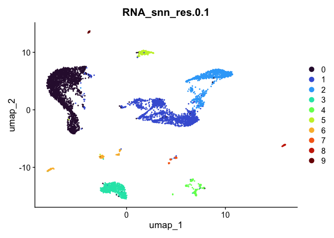
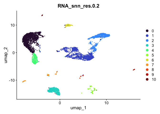
Visualize clustering
Dimensionality reduction plots can be used to visualize the clustering results. On these plots, we can see how each clustering resolution aligns with patterns in the data revealed by dimensionality reductions.
UMAP
# UMAP colored by cluster
lapply(cluster.resolutions, function(res){
  DimPlot(experiment.aggregate,
          group.by = res,
          reduction = "umap",
          shuffle = TRUE) +
    scale_color_viridis_d(option = "turbo")
})
## [[1]]
##
## [[2]]
##
## [[3]]

##
## [[4]]
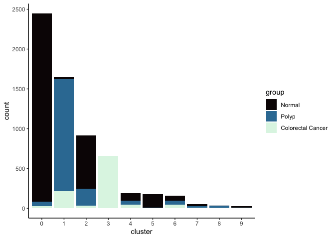
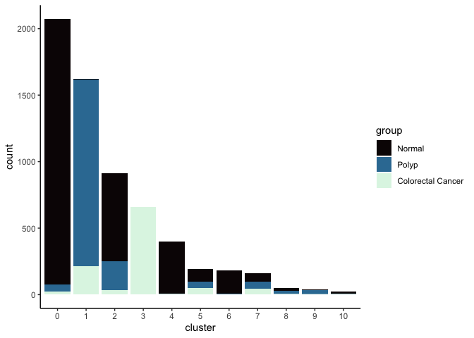
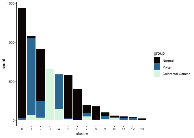
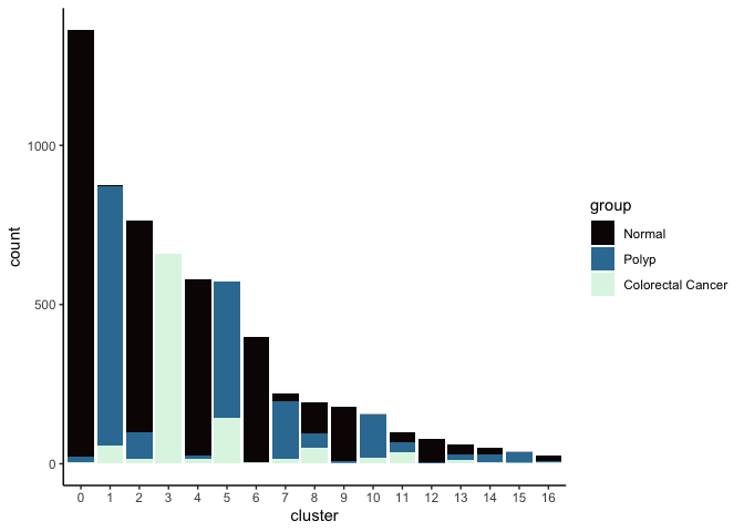
Investigate the relationship between cluster identity and sample identity
lapply(cluster.resolutions, function(res){
         tmp = experiment.aggregate@meta.data[,c(res, "group")]
         colnames(tmp) = c("cluster", "group")
         ggplot(tmp, aes(x = cluster, fill = group)) +
           geom_bar() +
           scale_fill_viridis_d(option = "mako") +
           theme_classic()
})
## [[1]]
##
## [[2]]
##
## [[3]]
##
## [[4]]
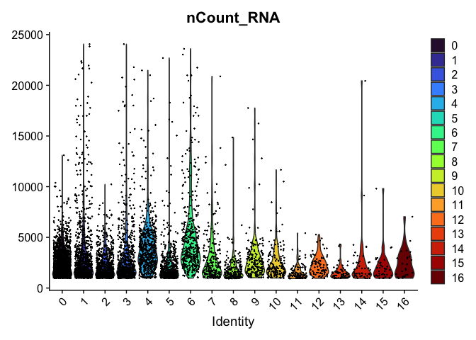
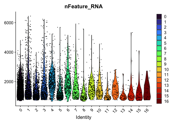
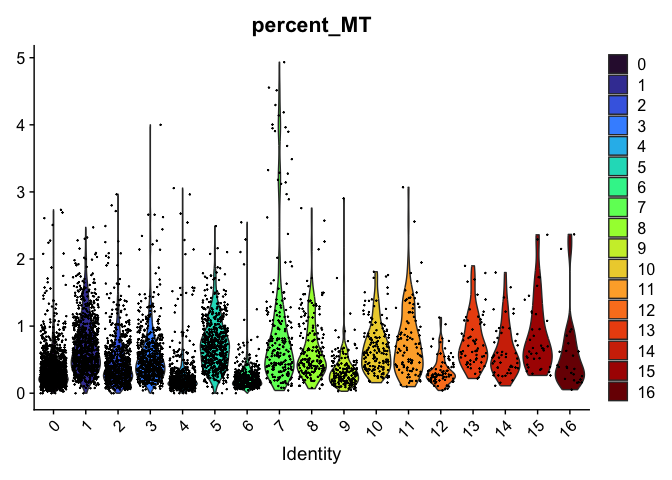
Investigate the relationship between cluster identity and metadata values
Here, example plots are displayed for the lowest resolution in order to save space. To see plots for each resolution, use lapply().
VlnPlot(experiment.aggregate,
        group.by = "RNA_snn_res.0.4",
        features = "nCount_RNA",
        pt.size = 0.1) +
  scale_fill_viridis_d(option = "turbo")
VlnPlot(experiment.aggregate,
        group.by = "RNA_snn_res.0.4",
        features = "nFeature_RNA",
        pt.size = 0.1) +
  scale_fill_viridis_d(option = "turbo")
VlnPlot(experiment.aggregate,
        group.by = "RNA_snn_res.0.4",
        features = "percent_MT",
        pt.size = 0.1) +
  scale_fill_viridis_d(option = "turbo")
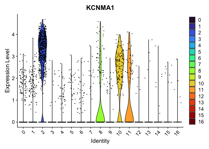
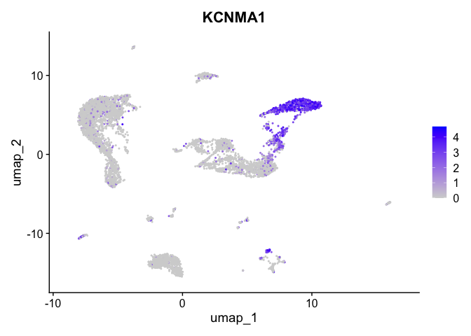
Visualize expression of genes of interest
FeaturePlot(experiment.aggregate,
            reduction = "umap",
            features = "KCNMA1")

VlnPlot(experiment.aggregate,
        group.by = "RNA_snn_res.0.4",
        features = "KCNMA1",
        pt.size = 0.1) +
  scale_fill_viridis_d(option = "turbo")
Select a resolution
For now, let’s use resolution 0.4. Over the remainder of this section, we will refine the clustering further.
Idents(experiment.aggregate) <- "RNA_snn_res.0.4"
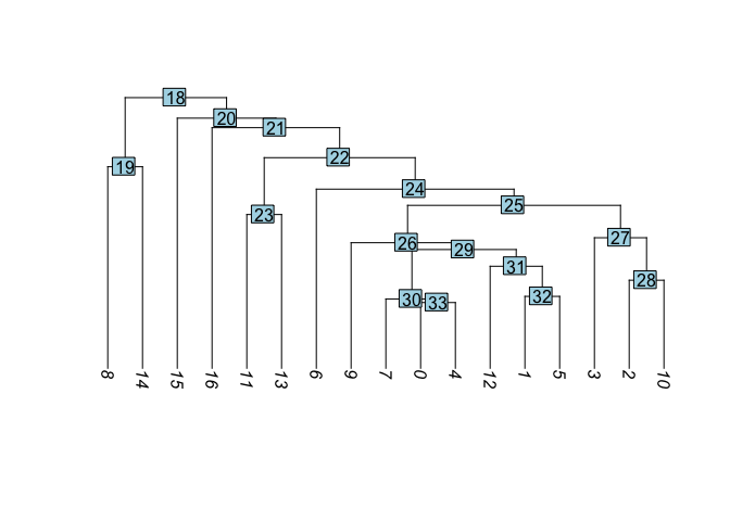
Visualize cluster tree
Building a phylogenetic tree relating the ‘average’ cell from each group in default ‘Ident’ (currently “RNA_snn_res.0.1”). This tree is estimated based on a distance matrix constructed in either gene expression space or PCA space.
experiment.aggregate <- BuildClusterTree(experiment.aggregate, dims = 1:50)
PlotClusterTree(experiment.aggregate)
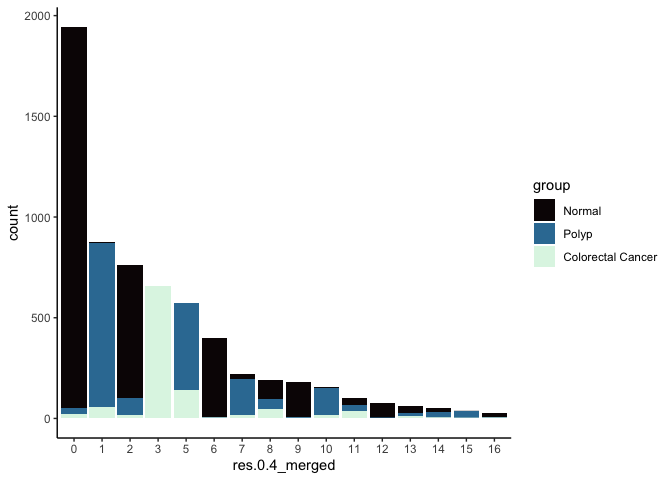
Merge clusters
In many experiments, the clustering resolution does not need to be uniform across all of the cell types present. While for some cell types of interest fine detail may be desirable, for others, simply grouping them into a larger parent cluster is sufficient. Merging cluster is very straightforward.
experiment.aggregate <- RenameIdents(experiment.aggregate,
                                     '4' = '0')
experiment.aggregate$res.0.4_merged <- Idents(experiment.aggregate)
table(experiment.aggregate$res.0.4_merged)
##
##    0    1    2    3    5    6    7    8    9   10   11   12   13   14   15   16
## 1944  875  764  658  574  399  222  193  180  154  100   79   60   51   37   25
experiment.aggregate@meta.data %>%
  ggplot(aes(x = res.0.4_merged, fill = group)) +
  geom_bar() +
  scale_fill_viridis_d(option = "mako") +
  theme_classic()
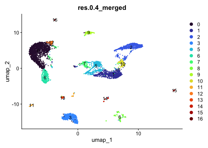
DimPlot(experiment.aggregate,
        reduction = "umap",
        group.by = "res.0.4_merged",
        label = TRUE) +
  scale_color_viridis_d(option = "turbo")
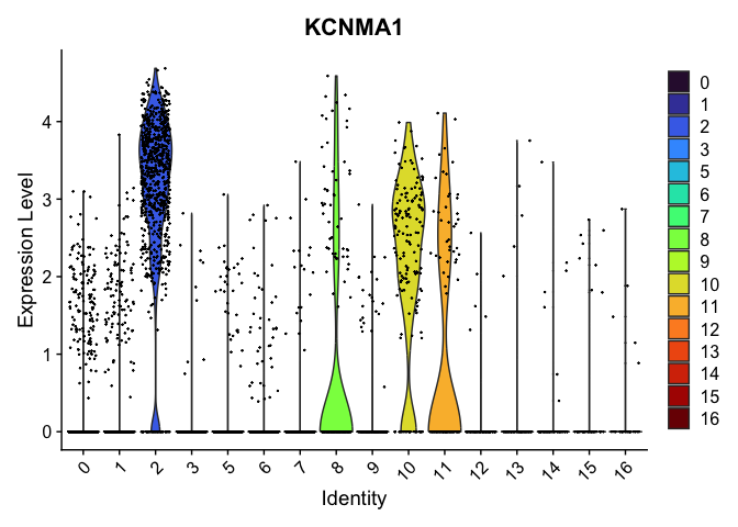
VlnPlot(experiment.aggregate,
        group.by = "res.0.4_merged",
        features = "KCNMA1") +
  scale_fill_viridis_d(option = "turbo")
Reorder the clusters
Merging the clusters changed the order in which they appear on a plot. In order to reorder the clusters for plotting purposes take a look at the levels of the identity, then re-level as desired.
levels(experiment.aggregate$res.0.4_merged)
##  [1] "0"  "1"  "2"  "3"  "5"  "6"  "7"  "8"  "9"  "10" "11" "12" "13" "14" "15"
## [16] "16"
# move one cluster to the first position
experiment.aggregate$res.0.4_merged <- relevel(experiment.aggregate$res.0.4_merged, "0")
levels(experiment.aggregate$res.0.4_merged)
##  [1] "0"  "1"  "2"  "3"  "5"  "6"  "7"  "8"  "9"  "10" "11" "12" "13" "14" "15"
## [16] "16"
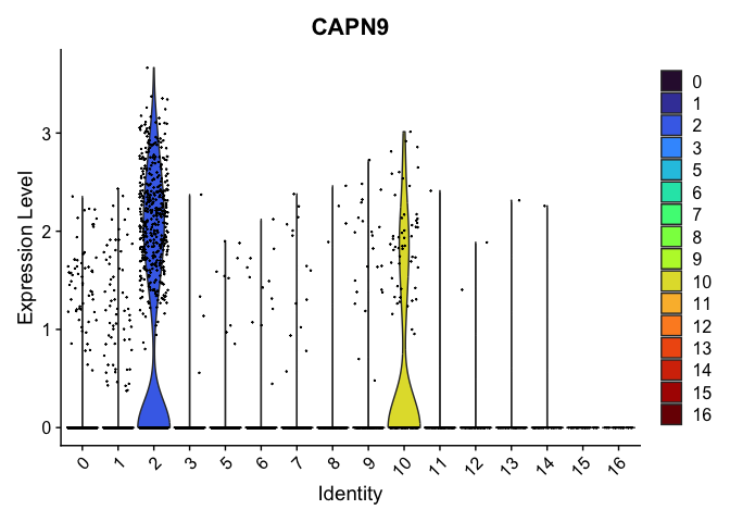
# the color assigned to some clusters will change
VlnPlot(experiment.aggregate,
        group.by = "res.0.4_merged",
        features = "CAPN9",
        pt.size = 0.1) +
  scale_fill_viridis_d(option = "turbo")
# re-level entire factor
new.order <- as.character(sort(as.numeric(levels(experiment.aggregate$res.0.4_merged))))
experiment.aggregate$res.0.4_merged <- factor(experiment.aggregate$res.0.4_merged, levels = new.order)
levels(experiment.aggregate$res.0.4_merged)
##  [1] "0"  "1"  "2"  "3"  "5"  "6"  "7"  "8"  "9"  "10" "11" "12" "13" "14" "15"
## [16] "16"
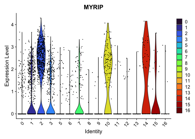
VlnPlot(experiment.aggregate,
        group.by = "res.0.4_merged",
        features = "MYRIP",
        pt.size = 0.1) +
  scale_fill_viridis_d(option = "turbo")
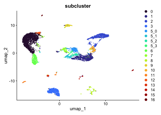
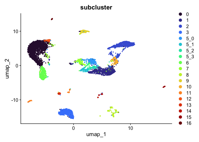
Subcluster
While merging clusters reduces the resolution in some parts of the experiment, sub-clustering has the opposite effect. Let’s produce sub-clusters for cluster 5.
experiment.aggregate <- FindSubCluster(experiment.aggregate,
                                       graph.name = "RNA_snn",
                                       cluster = 5,
                                       subcluster.name = "subcluster")
## Modularity Optimizer version 1.3.0 by Ludo Waltman and Nees Jan van Eck
##
## Number of nodes: 574
## Number of edges: 23790
##
## Running Louvain algorithm...
## Maximum modularity in 10 random starts: 0.7231
## Number of communities: 4
## Elapsed time: 0 seconds
experiment.aggregate$subcluster <- factor(experiment.aggregate$subcluster,
                                          levels = c(as.character(0:3),
                                                     "5_0", "5_1", "5_2", "5_3",
                                                     as.character(6:16)))
DimPlot(experiment.aggregate,
        reduction = "umap",
        group.by = "subcluster",
        shuffle = TRUE) +
  scale_color_viridis_d(option = "turbo")
sort(unique(experiment.aggregate$subcluster))
##  [1] 0   1   2   3   5_0 5_1 5_2 5_3 6   7   8   9   10  11  12  13  14  15  16
## Levels: 0 1 2 3 5_0 5_1 5_2 5_3 6 7 8 9 10 11 12 13 14 15 16
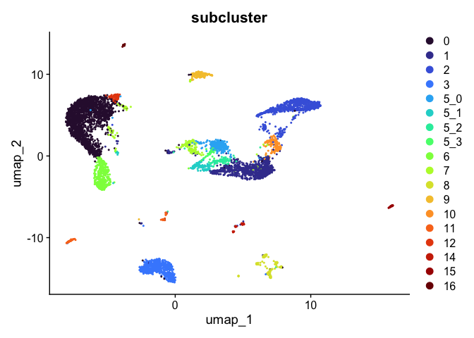
Subset experiment by cluster identity
After exploring and refining the cluster resolution, we may have identified some clusters that are composed of cells we aren’t interested in. For example, if we have identified a cluster likely composed of contaminants, this cluster can be removed from the analysis. Alternatively, if a group of clusters have been identified as particularly of interest, these can be isolated and re-analyzed.
# remove cluster 13
Idents(experiment.aggregate) <- experiment.aggregate$subcluster
experiment.tmp <- subset(experiment.aggregate, subcluster != "13")
DimPlot(experiment.tmp,
        reduction = "umap",
        group.by = "subcluster",
        shuffle = TRUE) +
  scale_color_viridis_d(option = "turbo")
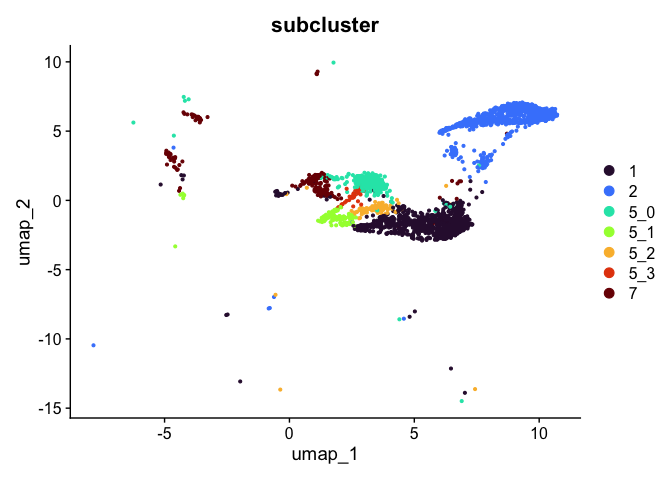
# retain cells belonging only to specified clusters
experiment.tmp <- subset(experiment.aggregate, subcluster %in% c("1", "2", "5_0", "5_1", "5_2", "5_3", "7"))
DimPlot(experiment.tmp,
        reduction = "umap",
        group.by = "subcluster",
        shuffle = TRUE) +
  scale_color_viridis_d(option = "turbo")
Identify marker genes
Seurat provides several functions that can help you find markers that define clusters via differential expression:
-
FindMarkersidentifies markers for a cluster relative to all other clusters -
FindAllMarkersperforms the find markers operation for all clusters -
FindAllMarkersNodedefines all markers that split a node from the cluster tree
FindMarkers
markers <- FindMarkers(experiment.aggregate,
                       group.by = "subcluster",
                       ident.1 = "1")
length(which(markers$p_val_adj < 0.05)) # how many are significant?
## [1] 3023
head(markers) %>%
  kable() %>%
  kable_styling("striped")
| p_val | avg_log2FC | pct.1 | pct.2 | p_val_adj | |
|---|---|---|---|---|---|
| CEMIP | 0 | 4.050263 | 0.624 | 0.070 | 0 |
| EDAR | 0 | 4.164535 | 0.393 | 0.030 | 0 |
| CASC19 | 0 | 3.181330 | 0.557 | 0.088 | 0 |
| NKD1 | 0 | 3.075292 | 0.551 | 0.093 | 0 |
| GRM8 | 0 | 2.650081 | 0.613 | 0.116 | 0 |
| AGBL4 | 0 | 2.578523 | 0.584 | 0.119 | 0 |
The “pct.1” and “pct.2” columns record the proportion of cells with normalized expression above 0 in ident.1 and ident.2, respectively. The “p_val” is the raw p-value associated with the differential expression test, while the BH-adjusted value is found in “p_val_adj”. Finally, “avg_logFC” is the average log fold change difference between the two groups.
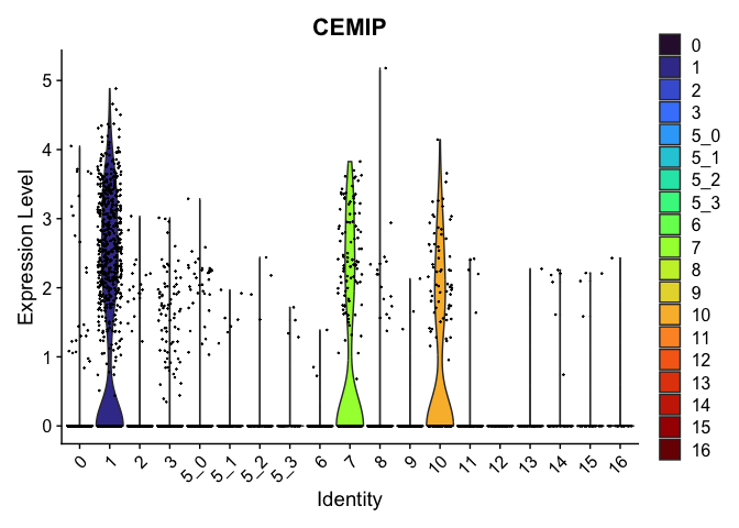
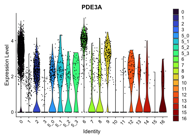
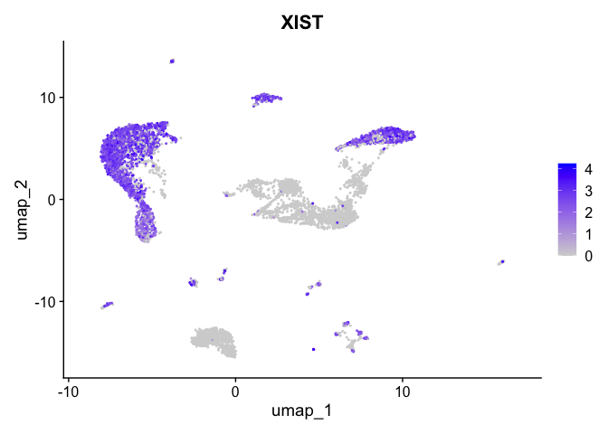
Marker genes identified this way can be visualized in violin plots, feature plots, and heat maps.
view.markers <- c(rownames(markers[markers$avg_log2FC > 0,])[1],
                  rownames(markers[markers$avg_log2FC < 0,])[1])
lapply(view.markers, function(marker){
  VlnPlot(experiment.aggregate,
          group.by = "subcluster",
          features = marker) +
    scale_fill_viridis_d(option = "turbo")
})
## [[1]]
##
## [[2]]
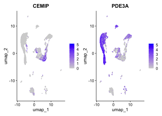
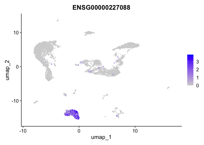
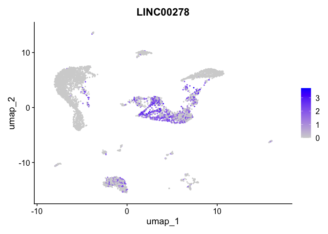
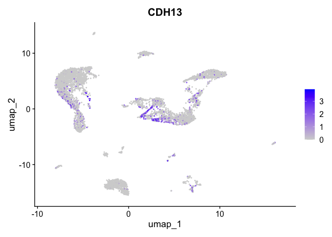
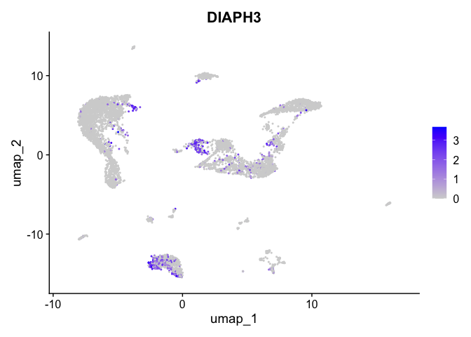
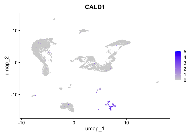
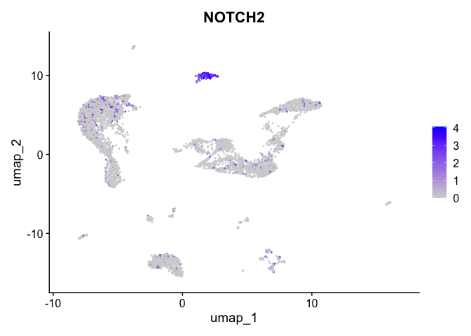
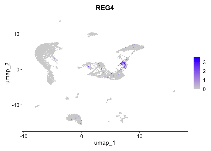
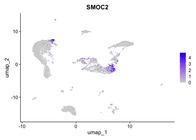
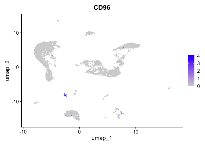
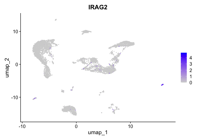
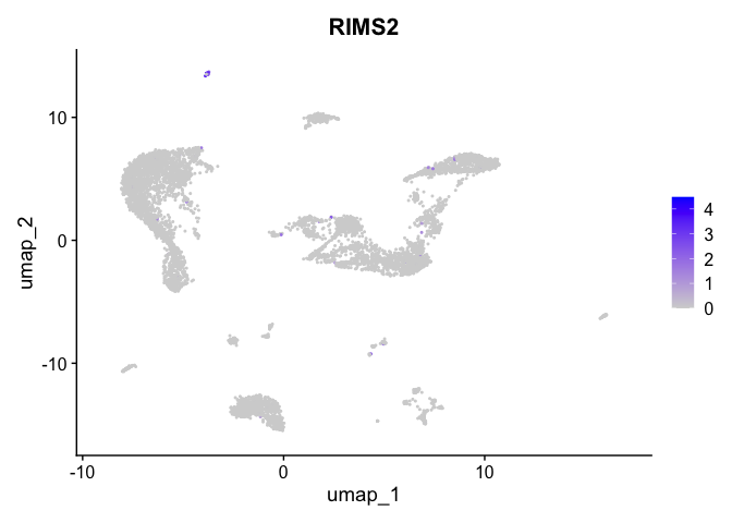
FeaturePlot(experiment.aggregate,
            features = view.markers,
            ncol = 2)
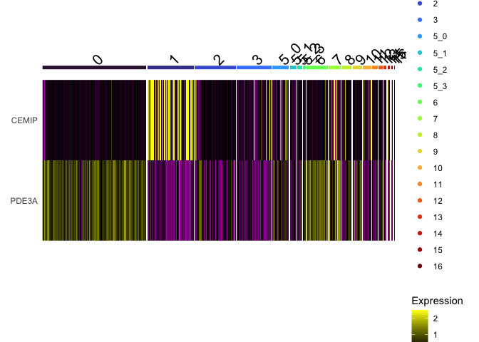
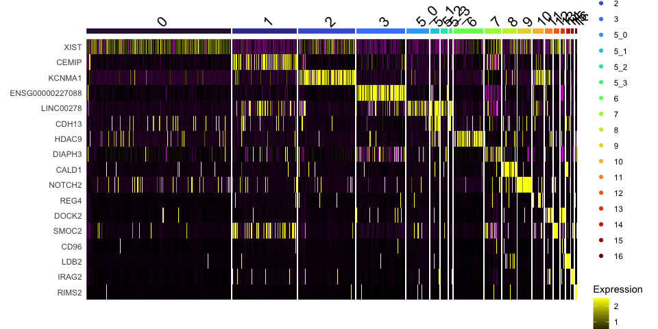
DoHeatmap(experiment.aggregate,
          group.by = "subcluster",
          features = view.markers,
          group.colors = viridis::turbo(length(levels(experiment.aggregate$subcluster))))
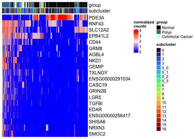
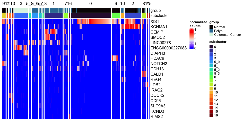
Improved heatmap
The Seurat DoHeatmap function provided by Seurat provides a convenient look at expression of selected genes. The ComplexHeatmap library generates heat maps with a much finer level of control.
cluster.colors <- viridis::turbo(length(levels(experiment.aggregate$subcluster)))
names(cluster.colors) <- levels(experiment.aggregate$subcluster)
group.colors <- viridis::mako(length(levels(experiment.aggregate$group)))
names(group.colors) <- levels(experiment.aggregate$group)
top.annotation <- columnAnnotation(df = experiment.aggregate@meta.data[,c("group", "subcluster")],
                                   col = list(group = group.colors,
                                              subcluster = cluster.colors))
mat <- as.matrix(GetAssayData(experiment.aggregate[rownames(markers)[1:20],],
                              slot = "data"))
Heatmap(mat,
        name = "normalized\ncounts",
        show_row_dend = FALSE,
        show_column_dend = FALSE,
        show_column_names = FALSE,
        top_annotation = top.annotation)
FindAllMarkers
FindAllMarkers can be used to automate this process across all clusters.
Idents(experiment.aggregate) <- "subcluster"
markers <- FindAllMarkers(experiment.aggregate,
                          only.pos = TRUE,
                          min.pct = 0.25,
                          thresh.use = 0.25)
tapply(markers$p_val_adj, markers$cluster, function(x){
  length(x < 0.05)
})
##    0    1    2    3  5_0  5_1  5_2  5_3    6    7    8    9   10   11   12   13
## 1193 1315  533 1462  269  783  231  339 1627  693  320  583  509  291  335  296
##   14   15   16
##  404  279  272
head(markers) %>%
  kable() %>%
  kable_styling("striped")
| p_val | avg_log2FC | pct.1 | pct.2 | p_val_adj | cluster | gene | |
|---|---|---|---|---|---|---|---|
| XIST | 0 | 1.713669 | 0.861 | 0.292 | 0 | 0 | XIST |
| SCNN1B | 0 | 1.729461 | 0.787 | 0.273 | 0 | 0 | SCNN1B |
| PDE3A | 0 | 1.751226 | 0.938 | 0.428 | 0 | 0 | PDE3A |
| NR5A2 | 0 | 1.918904 | 0.781 | 0.311 | 0 | 0 | NR5A2 |
| SELENBP1 | 0 | 1.881164 | 0.796 | 0.331 | 0 | 0 | SELENBP1 |
| PPARGC1A | 0 | 2.246897 | 0.706 | 0.251 | 0 | 0 | PPARGC1A |
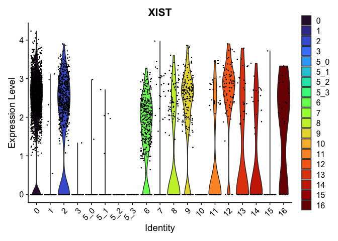
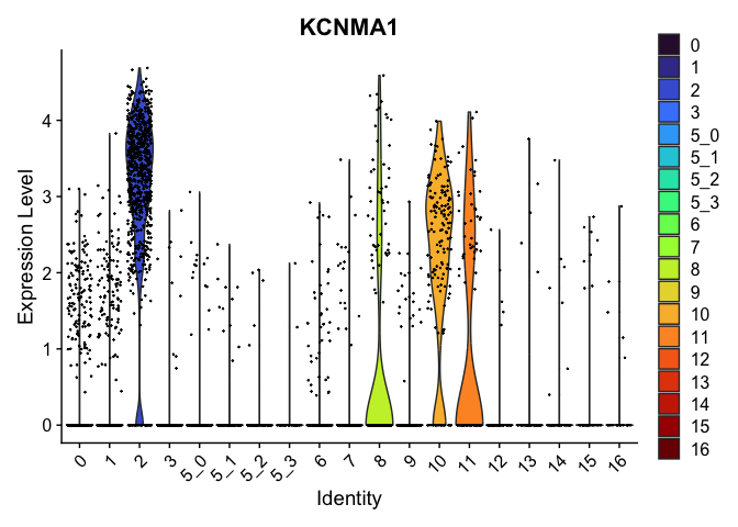
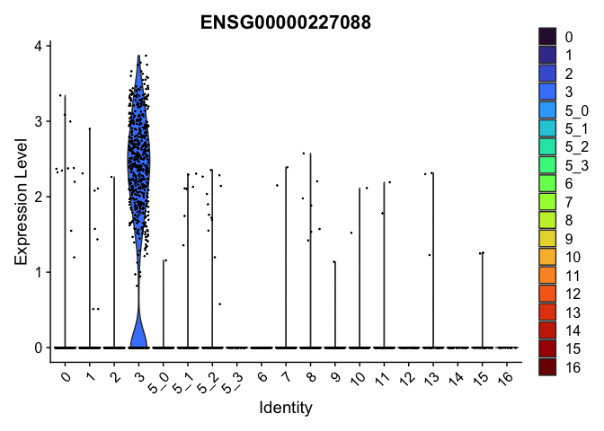
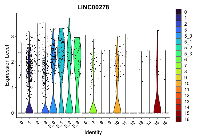
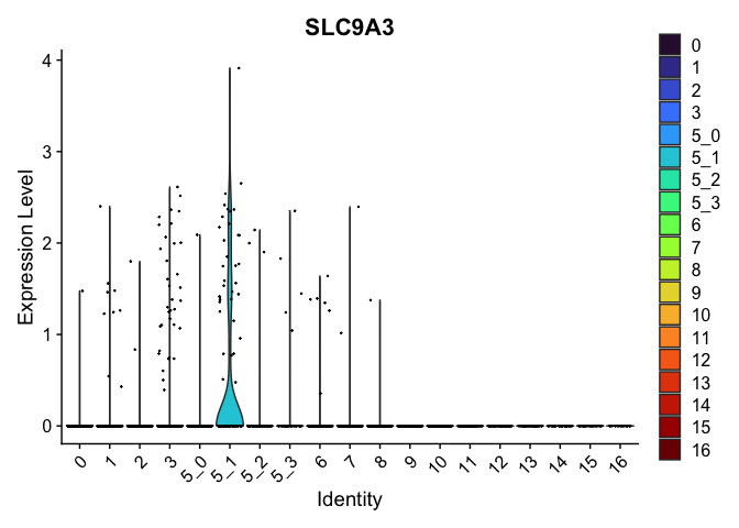
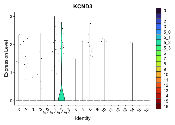
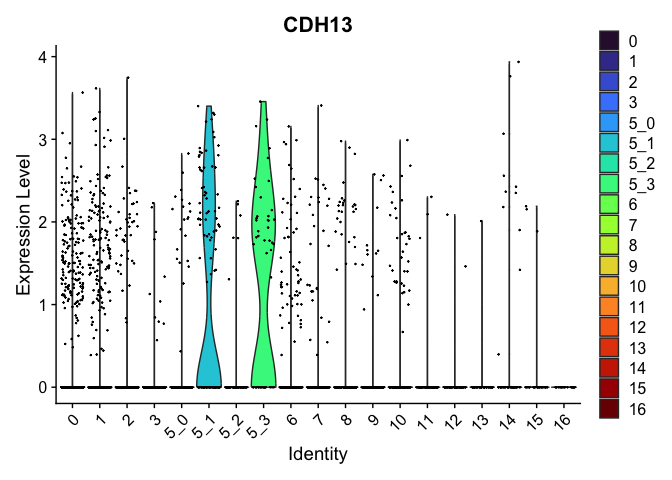
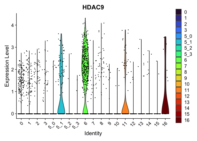
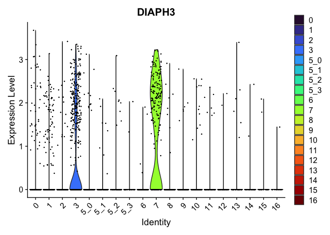
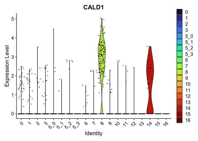
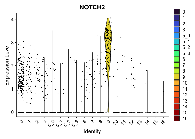
view.markers <- tapply(markers$gene, markers$cluster, function(x){head(x,1)})
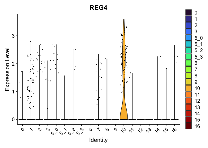
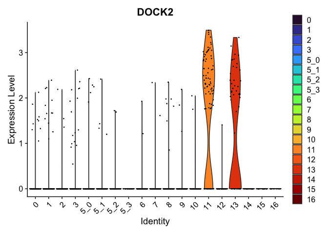
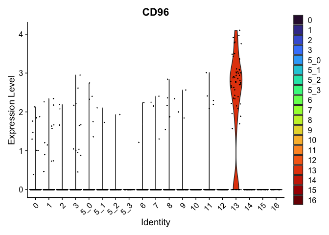
# violin plots
lapply(view.markers, function(marker){
VlnPlot(experiment.aggregate,
group.by = "subcluster",
features = marker) +
scale_fill_viridis_d(option = "turbo")
})
## $`0`
##
## $`1`

##
## $`2`
##
## $`3`
##
## $`5_0`
##
## $`5_1`
##
## $`5_2`
##
## $`5_3`
##
## $`6`
##
## $`7`
##
## $`8`
##
## $`9`
##
## $`10`
##
## $`11`
##
## $`12`
##
## $`13`
##
## $`14`
##
## $`15`
##
## $`16`
# feature plots
lapply(view.markers, function(marker){
  FeaturePlot(experiment.aggregate,
              features = marker)
})
## $`0`
##
## $`1`

##
## $`2`
##
## $`3`
##
## $`5_0`
##
## $`5_1`

##
## $`5_2`

##
## $`5_3`
##
## $`6`

##
## $`7`
##
## $`8`
##
## $`9`
##
## $`10`
##
## $`11`

##
## $`12`
##
## $`13`
##
## $`14`

##
## $`15`
##
## $`16`
# heat map
DoHeatmap(experiment.aggregate,
          group.by = "subcluster",
          features = view.markers,
          group.colors = viridis::turbo(length(unique(experiment.aggregate$subcluster))))
# ComplexHeatmap
mat <- as.matrix(GetAssayData(experiment.aggregate[view.markers,],
                              slot = "data"))
Heatmap(mat,
        name = "normalized\ncounts",
        show_row_dend = FALSE,
        show_column_dend = FALSE,
        show_column_names = FALSE,
        column_split = experiment.aggregate$subcluster,
        top_annotation = top.annotation)
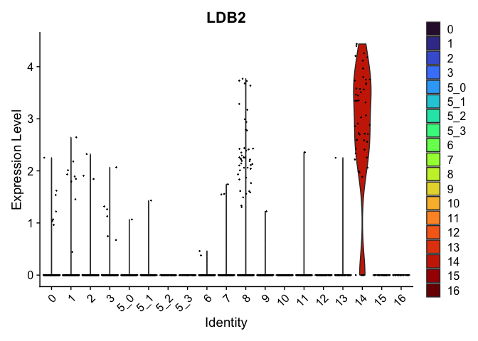
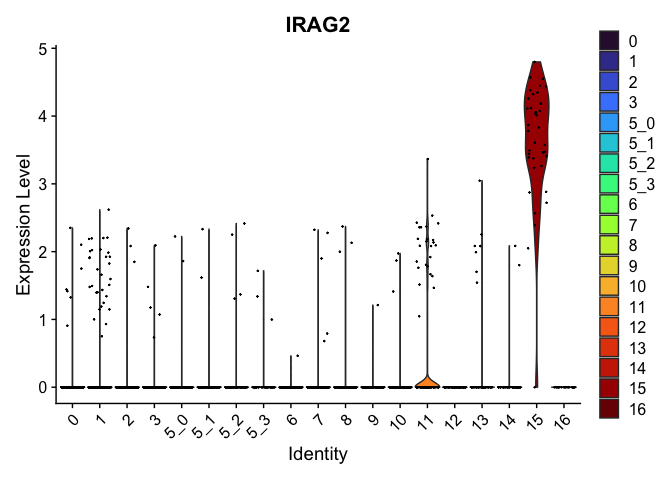
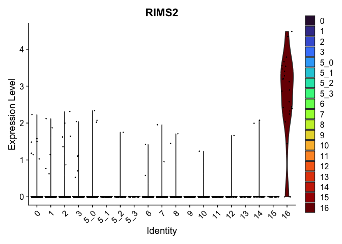
Calculate mean marker expression within clusters
You may want to get an idea of the mean expression of markers in a cluster or group of clusters. The percent expressing is provided by FindMarkers and FindAllMarkers, along with the average log fold change, but not the expression value itself. The function below calculates a mean for the supplied marker in the named cluster(s) and all other groups. Please note that this function accesses the active identity.
# ensure active identity is set to desired clustering resolution
Idents(experiment.aggregate) <- experiment.aggregate$subcluster
# define function
getGeneClusterMeans <- function(feature, idents){
x = GetAssayData(experiment.aggregate)[feature,]
m = tapply(x, Idents(experiment.aggregate) %in% idents, mean)
names(m) = c("mean.out.of.idents", "mean.in.idents")
return(m[c(2,1)])
}
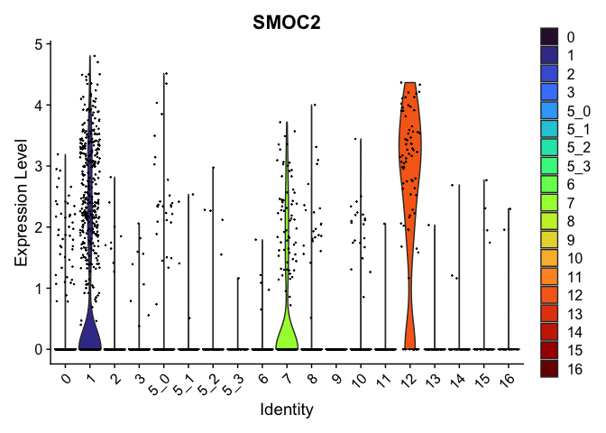
# calculate means for a single marker
getGeneClusterMeans("SMOC2", c("1"))
##     mean.in.idents mean.out.of.idents
##           1.017707           0.122972
# add means to marker table (example using subset)
markers.small <- markers[view.markers,]
means <- matrix(mapply(getGeneClusterMeans, view.markers, markers.small$cluster), ncol = 2, byrow = TRUE)
colnames(means) <- c("mean.in.cluster", "mean.out.of.cluster")
rownames(means) <- view.markers
markers.small <- cbind(markers.small, means)
markers.small[,c("cluster", "mean.in.cluster", "mean.out.of.cluster", "avg_log2FC", "p_val_adj")] %>%
  kable() %>%
  kable_styling("striped")
| cluster | mean.in.cluster | mean.out.of.cluster | avg_log2FC | p_val_adj | |
|---|---|---|---|---|---|
| XIST | 0 | 2.2101441 | 0.7100777 | 1.713669 | 0 |
| CEMIP | 1 | 1.6711633 | 0.1454736 | 4.050263 | 0 |
| KCNMA1 | 2 | 3.0963487 | 0.2346476 | 4.714387 | 0 |
| ENSG00000227088 | 3 | 1.9809564 | 0.0204090 | 7.106729 | 0 |
| LINC00278 | 1 | 0.7598408 | 0.2831158 | 1.157253 | 0 |
| SLC9A3 | 5_1 | 0.5027155 | 0.0153786 | 5.439006 | 0 |
| KCND3 | 5_2 | 0.5073249 | 0.0166944 | 4.994722 | 0 |
| CDH13 | 5_1 | 1.0908523 | 0.1689067 | 3.118900 | 0 |
| HDAC9 | 5_1 | 0.9552779 | 0.2454293 | 2.019423 | 0 |
| DIAPH3 | 3 | 0.6905352 | 0.1227073 | 2.505526 | 0 |
| CALD1 | 8 | 2.7860202 | 0.0431066 | 7.177446 | 0 |
| NOTCH2 | 9 | 2.7695987 | 0.1427036 | 5.561178 | 0 |
| REG4 | 10 | 0.9806473 | 0.0306120 | 5.588265 | 0 |
| DOCK2 | 11 | 1.7406667 | 0.0308358 | 6.362020 | 0 |
| SMOC2 | 1 | 1.0177069 | 0.1229720 | 3.327579 | 0 |
| CD96 | 13 | 2.2774955 | 0.0181706 | 7.954007 | 0 |
| LDB2 | 14 | 2.8090358 | 0.0257107 | 7.840347 | 0 |
| IRAG2 | 11 | 0.5138023 | 0.0431771 | 2.484657 | 0 |
| RIMS2 | 16 | 2.6669021 | 0.0087764 | 9.897168 | 0 |
Advanced visualizations
Researchers may use the tree, markers, domain knowledge, and goals to identify useful clusters. This may mean adjusting PCA to use, choosing a new resolution, merging clusters together, sub-clustering, sub-setting, etc. You may also want to use automated cell type identification at this point, which will be discussed in the next section.
Address overplotting
Single cell and single nucleus experiments may include so many cells that dimensionality reduction plots sometimes suffer from overplotting, where individual points are difficult to see. The following code addresses this by adjusting the size and opacity of the points.
alpha.use <- 0.4
p <- DimPlot(experiment.aggregate,
             group.by="subcluster",
             pt.size=0.5,
             reduction = "umap",
             shuffle = TRUE) +
  scale_color_viridis_d(option = "turbo")
p$layers[[1]]$mapping$alpha <- alpha.use
p + scale_alpha_continuous(range = alpha.use, guide = FALSE)
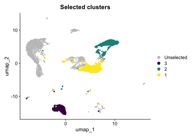
Highlight a subset
DimPlot(experiment.aggregate,
        group.by = "subcluster",
        cells.highlight = CellsByIdentities(experiment.aggregate, idents = c("1", "2", "3")),
        cols.highlight = c(viridis::viridis(3))) +
  ggtitle("Selected clusters")
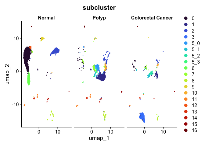
Split dimensionality reduction plots
DimPlot(experiment.aggregate,
        group.by = "subcluster",
        split.by = "group") +
  scale_color_viridis_d(option = "turbo")
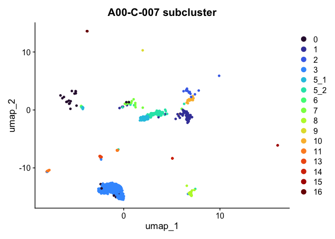
Plot a subset of cells
Note that the object itself is unchanged by the subsetting operation.
DimPlot(experiment.aggregate,
        group.by = "subcluster",
        reduction = "umap",
        cells = Cells(experiment.aggregate)[experiment.aggregate$orig.ident %in% "A001-C-007"]) +
  scale_color_viridis_d(option = "turbo") +
  ggtitle("A00-C-007 subcluster")
Automated cell type detection
ScType is one of many available automated cell type detection algorithms. It has the advantage of being fast and flexible; it can be used with the large human and mouse cell type database provided by the authors, with a user-defined database, or with some combination of the two.
In this section, we will use ScType to assign our clusters from Seurat to a cell type based on a hierarchical external database. The database supplied with the package is human but users can supply their own data. More details are available on Github.
Source ScType functions from Github
The source() functions in the code box below run scripts stored in the ScType GitHub repository. These scripts add two additional functions, gene_sets_prepare() and sctype_score(), to the global environment.
source("https://raw.githubusercontent.com/IanevskiAleksandr/sc-type/master/R/gene_sets_prepare.R")
source("https://raw.githubusercontent.com/IanevskiAleksandr/sc-type/master/R/sctype_score_.R")
Create marker database
The authors of ScType have provided an extensive database of human and mouse cell type markers in the following tissues:
- Immune system
- Pancreas
- Liver
- Eye
- Kidney
- Brain
- Lung
- Adrenal
- Heart
- Intestine
- Muscle
- Placenta
- Spleen
- Stomach
- Thymus
To set up the database for ScType, we run the gene_sets_prepare() function on a URL pointing to the full database, specifying the tissue subset to retrieve.
db.URL <- "https://raw.githubusercontent.com/IanevskiAleksandr/sc-type/master/ScTypeDB_full.xlsx"
tissue <- "Intestine"
gs.list <- gene_sets_prepare(db.URL, cell_type = "Intestine")
View(gs.list)
The database is composed of two lists (negative and positive) of cell type markers for the specified tissue. In this case, no negative markers have been provided, so the vectors of gene names in that part of the database are empty (length 0).
In addition to using the database supplied with the package, or substituting another database, it is possible to augment the provided database by changing the provided markers for an existing cell type, or adding another cell type to the object.
Let’s add a cell type and associated markers (markers from PanglaoDB).
gs.list$gs_positive$`Tuft cells` <- c("SUCNR1", "FABP1", "POU2F3", "SIGLECF", "CDHR2", "AVIL", "ESPN", "LRMP", "TRPM5", "DCLK1", "TAS1R3", "SOX9", "TUBB5", "CAMK2B", "GNAT3", "IL25", "PLCB2", "GFI1B", "ATOH1", "CD24A", "ASIC5", "KLF3", "KLF6", "DRD3", "NRADD", "GNG13", "NREP", "RGS2", "RAC2", "PTGS1", "IRF7", "FFAR3", "ALOX5", "TSLP", "IL4RA", "IL13RA1", "IL17RB", "PTPRC")
gs.list$gs_negative$`Tuft cells` <- NULL
Score cells
ScType scores every cell, summarizing the transformed and weighted expression of markers for each cell type. This generates a matrix with the dimensions cell types x cells.
es.max <- sctype_score(GetAssayData(experiment.aggregate, layer = "scale"),
                       scaled = TRUE,
                       gs = gs.list$gs_positive,
                       gs2 = gs.list$gs_negative)
# cell type scores of first cell
es.max[,1]
##         Smooth muscle cells              Lymphoid cells
##                  -0.3596284                  -0.1115503
## Intestinal epithelial cells                    ENS glia
##                  -0.4529272                  -0.1377867
##  Vascular endothelial cells               Stromal cells
##                  -0.1021364                  -0.1612953
## Lymphatic endothelial cells                  Tuft cells
##                   2.1633843                   0.7126830
Score clusters
The “ScType score” of each cluster is calculated by summing the cell-level scores within each cluster. The cell type with the largest (positive) score is the most highly enriched cell type for that cluster.
clusters <- sort(unique(experiment.aggregate$subcluster))
tmp <- lapply(clusters, function(cluster){
  es.max.cluster = sort(rowSums(es.max[, experiment.aggregate$subcluster == cluster]), decreasing = TRUE)
  out = head(data.frame(subcluster = cluster,
                        ScType = names(es.max.cluster),
                        scores = es.max.cluster,
                        ncells = sum(experiment.aggregate$subcluster == cluster)))
  out$rank = 1:length(out$scores)
  return(out)
})
cluster.ScType <- do.call("rbind", tmp)
cluster.ScType %>%
  pivot_wider(id_cols = subcluster,
              names_from = ScType,
              values_from = scores) %>%
  kable() %>%
  kable_styling(bootstrap_options = c("striped"), fixed_thead = TRUE)
| subcluster | Lymphatic endothelial cells | ENS glia | Lymphoid cells | Stromal cells | Vascular endothelial cells | Smooth muscle cells | Intestinal epithelial cells | Tuft cells |
|---|---|---|---|---|---|---|---|---|
| 0 | 195.3592499 | -80.0907487 | -125.8295023 | -154.744953 | -163.3416069 | -308.700705 | NA | NA |
| 1 | -23.5091750 | 38.5714704 | -39.7142237 | -90.642861 | -44.6501467 | NA | -40.527065 | NA |
| 2 | NA | -16.0594898 | -67.4117468 | -86.399911 | -42.8565375 | 165.963781 | NA | 282.663857 |
| 3 | NA | -15.2893895 | -19.7531236 | -28.330715 | 30.7432225 | -7.704916 | 139.124387 | NA |
| 5_0 | 0.5665667 | 0.4910627 | -29.0221662 | -48.314152 | -32.3981223 | NA | -94.637951 | NA |
| 5_1 | 10.8146520 | NA | 4.5434425 | -8.913896 | -8.3977374 | NA | 79.172784 | 28.591158 |
| 5_2 | -17.6516579 | -6.0084065 | -5.4276554 | -6.910908 | -9.3271656 | NA | -7.744006 | NA |
| 5_3 | 26.5719754 | -7.2671514 | -6.0062536 | -7.306450 | -5.1087651 | NA | NA | -12.913968 |
| 6 | 84.5148675 | NA | -13.5521554 | -28.216546 | -36.6926671 | NA | 258.908291 | 247.958134 |
| 7 | 38.4993114 | 12.6613201 | NA | -31.180464 | -11.8465241 | -5.162839 | NA | 30.476883 |
| 8 | 33.5529602 | 18.3513659 | 0.5603312 | 538.845499 | 23.4446944 | 510.701600 | NA | NA |
| 9 | NA | 9.8062122 | -11.5270313 | -17.694649 | -2.6660638 | NA | 546.525733 | -26.681074 |
| 10 | NA | 1.1565236 | -18.9557577 | -8.319629 | -15.3652684 | 95.063943 | NA | -10.310030 |
| 11 | NA | 4.2974245 | -0.7037958 | -10.826832 | 28.6889070 | -26.642138 | NA | 79.481078 |
| 12 | 16.8617145 | 17.4928064 | -7.9169431 | NA | 5.3327396 | 19.480815 | NA | -8.932543 |
| 13 | 11.3321455 | 15.8081143 | 328.7004295 | -10.546189 | -0.8110521 | NA | NA | 65.507083 |
| 14 | 7.2797743 | 18.5154041 | -6.4068253 | -8.001712 | 223.9865706 | -11.006069 | NA | NA |
| 15 | NA | 27.2964163 | 10.8899287 | -6.385268 | -3.9160561 | NA | -2.926101 | 242.841968 |
| 16 | -3.8282322 | -3.3227180 | -2.9070881 | -3.589013 | -2.5978425 | -7.873948 | NA | NA |
cluster.ScType.top <- cluster.ScType %>%
  filter(rank == 1) %>%
  select(subcluster, ncells, ScType, scores)
rownames(cluster.ScType.top) <- cluster.ScType.top$subcluster
cluster.ScType.top <- cluster.ScType.top %>%
  rename("score" = scores)
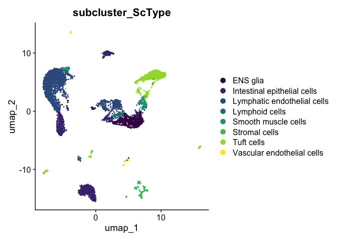
Once the scores have been calculated for each cluster, they can be added to the Seurat object.
subcluster.ScType <- cluster.ScType.top[experiment.aggregate$subcluster, "ScType"]
experiment.aggregate <- AddMetaData(experiment.aggregate,
                                    metadata = subcluster.ScType,
                                    col.name = "subcluster_ScType")
DimPlot(experiment.aggregate,
        reduction = "umap",
        group.by = "subcluster_ScType",
        shuffle = TRUE) +
  scale_color_viridis_d()
The ScType developer suggests that assignments with a score less than (number of cells in cluster)/4 are low confidence and should be set to unknown:
cluster.ScType.top <- cluster.ScType.top %>%
  mutate(ScType_filtered = ifelse(score >= ncells / 4, ScType, "Unknown"))
subcluster.ScType.filtered <- cluster.ScType.top[experiment.aggregate$subcluster, "ScType_filtered"]
experiment.aggregate <- AddMetaData(experiment.aggregate,
                                    metadata = subcluster.ScType.filtered,
                                    col.name = "subcluster_ScType_filtered")
DimPlot(experiment.aggregate,
        reduction = "umap",
        group.by = "subcluster_ScType_filtered",
        shuffle = TRUE) +
  scale_color_viridis_d()
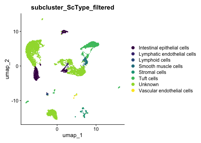
There is a large portion of the cells unassigned with a cell type. Could it be because of the cell types that we included from the database is not comprehensive? Based on the understanding that gut tract involves many immune related cell types, we are going to modify the procedure slightly to reflect this.
## prepare cell type marker database
source("https://raw.githubusercontent.com/ucdavis-bioinformatics-training/2025-July-Single-Cell-RNA-Seq-Analysis/main/software_scripts/scripts/mygene_sets_prepare.R")

gs.list.2tissues <- mygene_sets_prepare(db.URL, cell_type = c("Intestine", "Immune system"))

gs.list.2tissues$gs_positive$`Tuft cells` <- c("SUCNR1", "FABP1", "POU2F3", "SIGLECF", "CDHR2", "AVIL", "ESPN", "LRMP", "TRPM5", "DCLK1", "TAS1R3", "SOX9", "TUBB5", "CAMK2B", "GNAT3", "IL25", "PLCB2", "GFI1B", "ATOH1", "CD24A", "ASIC5", "KLF3", "KLF6", "DRD3", "NRADD", "GNG13", "NREP", "RGS2", "RAC2", "PTGS1", "IRF7", "FFAR3", "ALOX5", "TSLP", "IL4RA", "IL13RA1", "IL17RB", "PTPRC")
gs.list.2tissues$gs_negative$`Tuft cells` <- NULL

## calculate cell type marker scores
es.max <- sctype_score(GetAssayData(experiment.aggregate, layer = "scale"),
                       scaled = TRUE,
                       gs = gs.list.2tissues$gs_positive,
                       gs2 = gs.list.2tissues$gs_negative)

clusters <- sort(unique(experiment.aggregate$subcluster))
tmp <- lapply(clusters, function(cluster){
  es.max.cluster = sort(rowSums(es.max[, experiment.aggregate$subcluster == cluster]), decreasing = TRUE)
  out = head(data.frame(subcluster = cluster,
                        ScType = names(es.max.cluster),
                        scores = es.max.cluster,
                        ncells = sum(experiment.aggregate$subcluster == cluster)))
  out$rank = 1:length(out$scores)
  return(out)
})
cluster.ScType <- do.call("rbind", tmp)
cluster.ScType %>%
  pivot_wider(id_cols = subcluster,
              names_from = ScType,
              values_from = scores) %>%
  kable() %>%
  kable_styling(bootstrap_options = c("striped"), fixed_thead = TRUE)
| subcluster | Erythroid-like and erythroid precursor cells | Naive CD8+ T cells | Naive CD4+ T cells | Intermediate monocytes | Non-classical monocytes | Lymphatic endothelial cells | HSC/MPP cells | Cancer cells | Mast cells | Progenitor cells | Basophils | Granulocytes | Tuft cells | Smooth muscle cells | Macrophages | ENS glia | Classical Monocytes | Intestinal epithelial cells | Plasmacytoid Dendritic cells | Neutrophils | Myeloid Dendritic cells | Pro-B cells | Naive B cells | Memory B cells | Plasma B cells | Natural killer cells | Stromal cells | CD8+ NKT-like cells | CD4+ NKT-like cells | Memory CD8+ T cells | Memory CD4+ T cells | Effector CD8+ T cells | Effector CD4+ T cells | γδ-T cells | Endothelial | Platelets | Vascular endothelial cells | Pre-B cells |
|---|---|---|---|---|---|---|---|---|---|---|---|---|---|---|---|---|---|---|---|---|---|---|---|---|---|---|---|---|---|---|---|---|---|---|---|---|---|---|
| 0 | 500.9920 | 440.580357 | 440.58036 | 232.26130 | 198.12865 | 195.35925 | NA | NA | NA | NA | NA | NA | NA | NA | NA | NA | NA | NA | NA | NA | NA | NA | NA | NA | NA | NA | NA | NA | NA | NA | NA | NA | NA | NA | NA | NA | NA | NA |
| 1 | NA | NA | NA | NA | NA | NA | 379.33428 | 354.47997 | 351.73223 | 325.37737 | 322.927946 | 245.6994703 | NA | NA | NA | NA | NA | NA | NA | NA | NA | NA | NA | NA | NA | NA | NA | NA | NA | NA | NA | NA | NA | NA | NA | NA | NA | NA |
| 2 | NA | NA | NA | 29.61465 | 98.17102 | NA | NA | NA | NA | NA | NA | NA | 293.68800 | 165.96378 | 39.765612 | -16.05949 | NA | NA | NA | NA | NA | NA | NA | NA | NA | NA | NA | NA | NA | NA | NA | NA | NA | NA | NA | NA | NA | NA |
| 3 | NA | NA | NA | 45.44383 | NA | NA | NA | NA | NA | NA | NA | NA | NA | NA | NA | NA | 266.53755 | 139.12439 | 123.997771 | 112.94749 | 62.45649 | NA | NA | NA | NA | NA | NA | NA | NA | NA | NA | NA | NA | NA | NA | NA | NA | NA |
| 5_0 | NA | NA | NA | NA | NA | NA | 39.77159 | 17.84251 | 61.50933 | NA | NA | NA | NA | NA | 31.429771 | NA | NA | NA | NA | NA | NA | 33.345992 | 17.44173 | NA | NA | NA | NA | NA | NA | NA | NA | NA | NA | NA | NA | NA | NA | NA |
| 5_1 | NA | 51.054906 | 51.05491 | NA | NA | NA | 25.90200 | NA | NA | NA | NA | NA | 28.82644 | NA | NA | NA | NA | 79.17278 | NA | 22.72894 | NA | NA | NA | NA | NA | NA | NA | NA | NA | NA | NA | NA | NA | NA | NA | NA | NA | NA |
| 5_2 | NA | NA | NA | NA | NA | NA | NA | NA | NA | NA | NA | NA | NA | NA | 17.138196 | NA | 23.88967 | NA | NA | 36.26821 | NA | NA | 11.35855 | 11.35855 | 11.35855 | NA | NA | NA | NA | NA | NA | NA | NA | NA | NA | NA | NA | NA |
| 5_3 | NA | 6.555316 | NA | NA | NA | 26.57198 | 12.06027 | 11.89204 | 10.14403 | NA | NA | NA | NA | NA | NA | NA | NA | NA | NA | NA | NA | 8.714514 | NA | NA | NA | NA | NA | NA | NA | NA | NA | NA | NA | NA | NA | NA | NA | NA |
| 6 | NA | 132.533293 | 132.53329 | NA | 196.32896 | NA | 160.54721 | NA | NA | NA | NA | NA | 250.22050 | NA | NA | NA | NA | 258.90829 | NA | NA | NA | NA | NA | NA | NA | NA | NA | NA | NA | NA | NA | NA | NA | NA | NA | NA | NA | NA |
| 7 | NA | NA | NA | NA | NA | 38.49931 | 58.95581 | 21.05885 | NA | NA | 21.123324 | NA | 34.13761 | NA | NA | NA | NA | NA | NA | NA | NA | NA | NA | NA | NA | 22.05872 | NA | NA | NA | NA | NA | NA | NA | NA | NA | NA | NA | NA |
| 8 | NA | NA | NA | NA | NA | NA | NA | NA | NA | NA | NA | NA | NA | 510.70160 | NA | NA | NA | NA | NA | NA | 85.22016 | NA | NA | NA | NA | 239.14217 | 538.8455 | 169.6848 | 169.6848 | NA | NA | NA | NA | NA | NA | NA | NA | NA |
| 9 | NA | 51.842583 | 51.84258 | 16.40587 | 19.41742 | NA | NA | NA | NA | NA | NA | NA | NA | NA | 51.764699 | NA | NA | 546.52573 | NA | NA | NA | NA | NA | NA | NA | NA | NA | NA | NA | NA | NA | NA | NA | NA | NA | NA | NA | NA |
| 10 | NA | NA | NA | NA | NA | NA | 56.78168 | 36.59818 | NA | 33.76649 | NA | 15.4120101 | NA | 95.06394 | 9.246033 | NA | NA | NA | NA | NA | NA | NA | NA | NA | NA | NA | NA | NA | NA | NA | NA | NA | NA | NA | NA | NA | NA | NA |
| 11 | 220.9798 | NA | NA | NA | NA | NA | NA | NA | NA | NA | NA | NA | NA | NA | NA | NA | NA | NA | NA | NA | NA | NA | NA | NA | NA | NA | NA | NA | NA | 155.8204 | 155.8204 | 155.8204 | 155.8204 | 155.8204 | NA | NA | NA | NA |
| 12 | NA | NA | NA | 17.12134 | NA | 16.86171 | NA | NA | NA | NA | 19.564228 | NA | NA | 19.48081 | NA | 17.49281 | NA | NA | NA | NA | NA | 19.445712 | NA | NA | NA | NA | NA | NA | NA | NA | NA | NA | NA | NA | NA | NA | NA | NA |
| 13 | NA | 370.747066 | NA | NA | NA | NA | NA | NA | NA | NA | NA | NA | NA | NA | NA | NA | NA | NA | NA | NA | NA | NA | NA | NA | NA | NA | NA | NA | NA | 410.7221 | 410.7221 | 410.7221 | 410.7221 | 410.7221 | NA | NA | NA | NA |
| 14 | NA | NA | NA | NA | NA | NA | NA | NA | NA | 68.75233 | NA | NA | NA | NA | NA | NA | NA | NA | 95.532653 | NA | 119.53912 | NA | NA | NA | NA | NA | NA | NA | NA | NA | NA | NA | NA | NA | 334.4748 | 266.2053 | 219.1173 | NA |
| 15 | NA | NA | NA | NA | NA | NA | NA | NA | 154.59502 | NA | NA | NA | 243.47621 | NA | NA | 27.29642 | NA | NA | NA | NA | NA | NA | NA | NA | NA | 96.27992 | NA | 79.4633 | 79.4633 | NA | NA | NA | NA | NA | NA | NA | NA | NA |
| 16 | NA | NA | NA | NA | NA | NA | NA | NA | NA | NA | 3.184483 | 0.1212075 | NA | NA | NA | NA | NA | NA | 8.147396 | NA | 14.19179 | NA | NA | NA | NA | 4.41046 | NA | NA | NA | NA | NA | NA | NA | NA | NA | NA | NA | 0.3285586 |
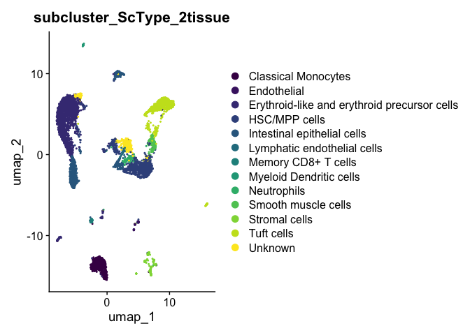
## Get the most likely cell type for each cluster
cluster.ScType.top <- cluster.ScType %>%
  filter(rank == 1) %>%
  select(subcluster, ncells, ScType, scores)
rownames(cluster.ScType.top) <- cluster.ScType.top$subcluster
cluster.ScType.top <- cluster.ScType.top %>%
  rename("score" = scores)

## filter new cell types and assign it to Seurat object
subcluster.ScType <- cluster.ScType.top[experiment.aggregate$subcluster, "ScType"]

cluster.ScType.top <- cluster.ScType.top %>%
  mutate(ScType_filtered = ifelse(score >= ncells / 4, ScType, "Unknown"))
subcluster.ScType.filtered <- cluster.ScType.top[experiment.aggregate$subcluster, "ScType_filtered"]
experiment.aggregate <- AddMetaData(experiment.aggregate,
                                    metadata = subcluster.ScType.filtered,
                                    col.name = "subcluster_ScType_2tissue")
DimPlot(experiment.aggregate,
        reduction = "umap",
        group.by = "subcluster_ScType_2tissue",
        shuffle = TRUE) +
  scale_color_viridis_d()
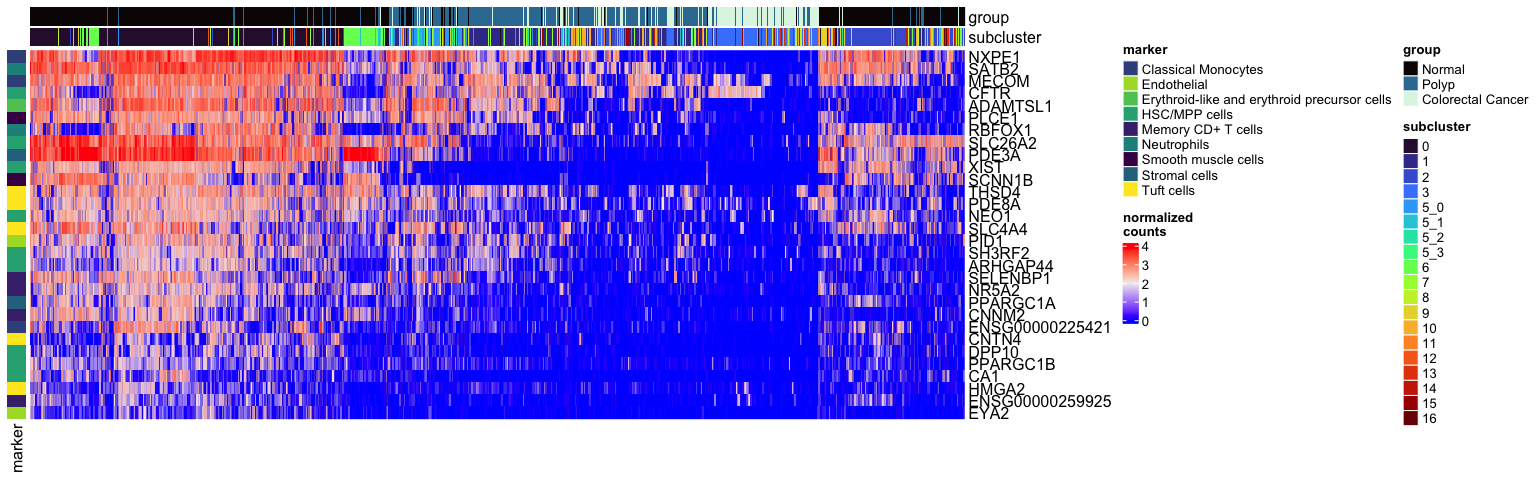
types <- grep("Unknown", unique(experiment.aggregate$subcluster_ScType_2tissue), value = TRUE, invert = TRUE)
type.markers <- unlist(lapply(gs.list.2tissues$gs_positive[types], function(m){
  rownames(markers[which(m %in% rownames(markers)),])
}))
type.markers <- type.markers[!duplicated(type.markers)]
type.markers.df <- data.frame(marker = type.markers,
                              type = gsub('[0-9]', '', names(type.markers)))
type.colors <- viridis::viridis(length(unique(type.markers.df$type)))
names(type.colors) <- unique(type.markers.df$type)
left.annotation <- rowAnnotation("marker" = type.markers.df$type, col = list(marker = type.colors))
mat <- as.matrix(GetAssayData(experiment.aggregate,
                              slot = "data")[type.markers.df$marker,])
Heatmap(mat,
        name = "normalized\ncounts",
        top_annotation = top.annotation,
        left_annotation = left.annotation,
        show_column_dend = FALSE,
        show_column_names = FALSE,
        show_row_dend = FALSE)
Cell type annotation using large language model (GPT-4)
Machine learning techniques have been an integrative part of bioinformatics work. In recent years, large language model and deep learning techniques have been applied to many fields, such as computer vision, text processing, …. Deep learning has been used in many areas of bioinformatics as well, such as Deepvariant for variant discovery, Dorado for signal processing to basecall Oxford Nanopore data, AlphaFold for protein structural prediction. Recently, one study assessed the ability of GPT models to annotate single cell data, GPTCelltype. It requires to have a subscription to query OpenAI API, so I ran the analysis. I am providing the results here so that you can compare it with the celltypes that we generated using marker genes.
First thing that I noticed is that I got slightly different results for the 3 times that I ran the analysis.
download.file("https://raw.githubusercontent.com/ucdavis-bioinformatics-training/2025-July-Single-Cell-RNA-Seq-Analysis/main/data_analysis/celltype.gpt.rds", "celltype.gpt.rds")
celltypes.gpt <- readRDS("celltype.gpt.rds")
kable(celltypes.gpt, 'html', align = 'c') %>% kable_styling(bootstrap_options = c("condensed", "responsive", "striped"))
| Analysis1 | Analysis2 | Analysis3 | |
|---|---|---|---|
| 0 | Pancreatic alpha cells | Osteoblasts | Parietal Cells |
| 1 | Intestinal stem cells | Intestinal Stem Cells | Intestinal Epithelial Cells |
| 2 | Goblet cells | Goblet Cells | Goblet Cells |
| 3 | Liver cells | Cancer Cells (Broad type, specific type unknown) | Tumor Cells |
| 5_0 | Testis cells | Prostate Cancer Cells | Tumor Cells |
| 5_1 | Colon cells | Colon Cells | Colon Cells |
| 5_2 | Duodenal cells | Pancreatic Cells | Small Intestinal Epithelial Cells |
| 5_3 | Heart cells | Heart Cells | Endothelial Cells |
| 6 | Cardiac cells | Liver Cells | Enterochromaffin Cells |
| 7 | Mitotic cells | Mitotic Cells (Broad type, specific type unknown) | Mitotic Cells |
| 8 | Mesenchymal cells | Endothelial Cells | Smooth Muscle Cells |
| 9 | Neural cells | Neuronal Cells | Neural Cells |
| 10 | Pancreatic cells | Enterocytes | Gastric Mucosa Cells |
| 11 | Immune cells | Immune Cells (Broad type, specific type unknown) | Immune Cells |
| 12 | Neurons | Neurons | Neurons |
| 13 | T cells | T Cells | T cells |
| 14 | Endothelial cells | Endothelial Cells | Endothelial Cells |
| 15 | Mucosal cells | B Cells | T cells |
| 16 | Neurons | Neurons | Neurons |
Prepare for the next section
Save the Seurat object and download the next Rmd file
# set the finalcluster to subcluster
experiment.aggregate$finalcluster <- experiment.aggregate$subcluster
# save object
saveRDS(experiment.aggregate, file="scRNA_workshop-05.rds")
Download the Rmd file
download.file("https://raw.githubusercontent.com/ucdavis-bioinformatics-training/2025-July-Single-Cell-RNA-Seq-Analysis/main/data_analysis/06-de_enrichment.Rmd", "06-de_enrichment.Rmd")
Session Information
sessionInfo()
## R version 4.4.3 (2025-02-28)
## Platform: aarch64-apple-darwin20
## Running under: macOS Ventura 13.7.1
##
## Matrix products: default
## BLAS:   /Library/Frameworks/R.framework/Versions/4.4-arm64/Resources/lib/libRblas.0.dylib
## LAPACK: /Library/Frameworks/R.framework/Versions/4.4-arm64/Resources/lib/libRlapack.dylib;  LAPACK version 3.12.0
##
## locale:
## [1] en_US.UTF-8/en_US.UTF-8/en_US.UTF-8/C/en_US.UTF-8/en_US.UTF-8
##
## time zone: America/Los_Angeles
## tzcode source: internal
##
## attached base packages:
## [1] grid      stats     graphics  grDevices utils     datasets  methods
## [8] base
##
## other attached packages:
## [1] ComplexHeatmap_2.20.0 HGNChelper_0.8.14     ggplot2_3.5.1
## [4] dplyr_1.1.4           tidyr_1.3.1           kableExtra_1.4.0
## [7] Seurat_5.2.1          SeuratObject_5.0.2    sp_2.1-4
##
## loaded via a namespace (and not attached):
##   [1] RColorBrewer_1.1-3     shape_1.4.6.1          rstudioapi_0.16.0
##   [4] jsonlite_1.8.8         magrittr_2.0.3         magick_2.8.5
##   [7] ggbeeswarm_0.7.2       spatstat.utils_3.1-2   farver_2.1.2
##  [10] rmarkdown_2.27         GlobalOptions_0.1.2    vctrs_0.6.5
##  [13] ROCR_1.0-11            Cairo_1.6-2            spatstat.explore_3.2-7
##  [16] htmltools_0.5.8.1      sass_0.4.9             sctransform_0.4.1
##  [19] parallelly_1.37.1      KernSmooth_2.23-26     bslib_0.7.0
##  [22] htmlwidgets_1.6.4      ica_1.0-3              plyr_1.8.9
##  [25] plotly_4.10.4          zoo_1.8-12             cachem_1.1.0
##  [28] igraph_2.0.3           mime_0.12              lifecycle_1.0.4
##  [31] iterators_1.0.14       pkgconfig_2.0.3        Matrix_1.7-2
##  [34] R6_2.5.1               fastmap_1.2.0          clue_0.3-65
##  [37] fitdistrplus_1.1-11    future_1.33.2          shiny_1.8.1.1
##  [40] digest_0.6.35          colorspace_2.1-0       S4Vectors_0.44.0
##  [43] patchwork_1.2.0        tensor_1.5             RSpectra_0.16-1
##  [46] irlba_2.3.5.1          labeling_0.4.3         progressr_0.14.0
##  [49] fansi_1.0.6            spatstat.sparse_3.0-3  httr_1.4.7
##  [52] polyclip_1.10-6        abind_1.4-5            compiler_4.4.3
##  [55] withr_3.0.0            doParallel_1.0.17      viridis_0.6.5
##  [58] fastDummies_1.7.3      highr_0.11             MASS_7.3-64
##  [61] rjson_0.2.21           tools_4.4.3            splitstackshape_1.4.8
##  [64] vipor_0.4.7            lmtest_0.9-40          ape_5.8
##  [67] beeswarm_0.4.0         zip_2.3.1              httpuv_1.6.15
##  [70] future.apply_1.11.2    goftest_1.2-3          glue_1.7.0
##  [73] nlme_3.1-167           promises_1.3.0         Rtsne_0.17
##  [76] cluster_2.1.8          reshape2_1.4.4         generics_0.1.3
##  [79] gtable_0.3.5           spatstat.data_3.0-4    data.table_1.15.4
##  [82] xml2_1.3.6             utf8_1.2.4             BiocGenerics_0.50.0
##  [85] spatstat.geom_3.2-9    RcppAnnoy_0.0.22       ggrepel_0.9.5
##  [88] RANN_2.6.1             foreach_1.5.2          pillar_1.9.0
##  [91] stringr_1.5.1          limma_3.60.2           spam_2.10-0
##  [94] RcppHNSW_0.6.0         later_1.3.2            circlize_0.4.16
##  [97] splines_4.4.3          lattice_0.22-6         survival_3.8-3
## [100] deldir_2.0-4           tidyselect_1.2.1       miniUI_0.1.1.1
## [103] pbapply_1.7-2          knitr_1.47             gridExtra_2.3
## [106] IRanges_2.38.0         svglite_2.1.3          scattermore_1.2
## [109] stats4_4.4.3           xfun_0.44              statmod_1.5.0
## [112] matrixStats_1.3.0      stringi_1.8.4          lazyeval_0.2.2
## [115] yaml_2.3.8             evaluate_0.23          codetools_0.2-20
## [118] tibble_3.2.1           cli_3.6.2              uwot_0.2.2
## [121] xtable_1.8-4           reticulate_1.39.0      systemfonts_1.1.0
## [124] munsell_0.5.1          jquerylib_0.1.4        Rcpp_1.0.12
## [127] globals_0.16.3         spatstat.random_3.2-3  png_0.1-8
## [130] ggrastr_1.0.2          parallel_4.4.3         presto_1.0.0
## [133] dotCall64_1.1-1        listenv_0.9.1          viridisLite_0.4.2
## [136] scales_1.3.0           ggridges_0.5.6         openxlsx_4.2.5.2
## [139] crayon_1.5.2           purrr_1.0.2            GetoptLong_1.0.5
## [142] rlang_1.1.3            cowplot_1.1.3