Last Updated March 25, 2021
Single Cell V(D)J Analysis with Seurat and some custom code!
Seurat is a popular R package that is designed for QC, analysis, and exploration of single cell data. Seurat aims to enable users to identify and interpret sources of heterogeneity from single cell transcriptomic measurements, and to integrate diverse types of single cell data. Further, the authors provide several tutorials on their website.
We start with loading needed libraries for R
Matt says we don’t need all the libraries
library(Seurat)
library(ggplot2)
library(knitr)
# I like this package
library(kableExtra)
library(cowplot)
library(dplyr)
library(circlize)
library(scales)
library(scRepertoire)
Load the Expression Matrix Data and create the combined base Seurat object.
Seurat provides a function Read10X to read in 10X data folder. First we read in data from each individual sample folder. Then, we initialize the Seurat object (CreateSeuratObject) with the raw (non-normalized data). Keep all genes expressed in >= 3 cells. Keep all cells with at least 200 detected genes. Also extracting sample names, calculating and adding in the metadata mitochondrial percentage of each cell. Some QA/QC Finally, saving the raw Seurat object.
Setup the experiment folder and data info
experiment_name = "Covid VDJ Example"
dataset_loc <- "./advsinglecellvdj_March2021"
ids <- c("T021PBMC", "T022PBMC")
ids
[1] "T021PBMC" "T022PBMC"
###1. Load the Cell Ranger Matrix Data (hdf5 file) and create the base Seurat object.
d10x.data <- lapply(ids, function(i){
  d10x <- Read10X_h5(file.path(dataset_loc,paste0(i,"_Counts/outs"),"raw_feature_bc_matrix.h5"))
  colnames(d10x) <- paste(sapply(strsplit(colnames(d10x),split="-"),'[[',1L),i,sep="-")
  d10x
})

names(d10x.data) <- ids
###2. Create the Seurat object
filter criteria: remove genes that do not occur in a minimum of 0 cells and remove cells that don’t have a minimum of 200 features
experiment.data <- do.call("cbind", d10x.data)

experiment.aggregate <- CreateSeuratObject(
  experiment.data,
  project = experiment_name,
  min.cells = 0,
  min.features = 300,
  names.field = 2,
  names.delim = "\\-")

experiment.aggregate
An object of class Seurat
36601 features across 13398 samples within 1 assay
Active assay: RNA (36601 features, 0 variable features)
###3. The percentage of reads that map to the mitochondrial genome
- Low-quality / dying cells often exhibit extensive mitochondrial contamination.
- We calculate mitochondrial QC metrics with the PercentageFeatureSet function, which calculates the percentage of counts originating from a set of features.
- We use the set of all genes, in mouse these genes can be identified as those that begin with ‘mt’, in human data they begin with MT.
experiment.aggregate$percent.mito <- PercentageFeatureSet(experiment.aggregate, pattern = "^MT-")
summary(experiment.aggregate$percent.mito)
Min. 1st Qu. Median Mean 3rd Qu. Max.
0.000 1.680 2.378 3.232 3.429 64.962
###4. QA/QC and filtering
# Custom violinplot code
violin_custom <- function(object, var, pt.size = 0.1, pt.alpha = 0.1, log = F){
	p <- ggplot(object[[]], aes(y = !!sym(var), x = orig.ident, fill = orig.ident)) +
	geom_violin(scale = "width", width = 0.9) +
	geom_point(position = position_jitterdodge(dodge.width = 0.9, jitter.width = 1.4),
		size = pt.size, alpha = pt.alpha) +
	labs(fill = NULL, x = "Identity", y = NULL, title = var) +
	cowplot::theme_cowplot() +
	theme(axis.text.x = element_text(angle = 45, hjust = 1), plot.title = element_text(hjust = 0.5))
	if (log){
		p <- p + scale_y_continuous(trans = "log10")
	}
	return(p)
}
Violin plot of genes/cell by sample:
var <- "nFeature_RNA"
violin_custom(experiment.aggregate, var)
Violin plot of nUMI by sample:
var <- "nCount_RNA"
violin_custom(experiment.aggregate, var, log=T) # Try Log = T
Violin plot of percent mitochondrial gene expression by sample:
var <- "percent.mito"
violin_custom(experiment.aggregate, var, log=T)
Warning: Transformation introduced infinite values in continuous y-axis
Warning: Transformation introduced infinite values in continuous y-axis
Warning: Removed 5 rows containing non-finite values (stat_ydensity).
Cell filtering
We use the information above to filter out cells. Here we choose those that have percent mitochondrial genes max of 8%, unique UMI counts under 3,000 or greater than 12,000 and contain at least 1000 features within them.
table(experiment.aggregate$orig.ident)
T021PBMC T022PBMC
8310 5088
experiment.aggregate <- subset(experiment.aggregate, percent.mito <= 8)

experiment.aggregate <- subset(experiment.aggregate, nCount_RNA >= 3000 & nCount_RNA <= 12000)

experiment.aggregate <- subset(experiment.aggregate, nFeature_RNA >= 1000)

experiment.aggregate
An object of class Seurat
36601 features across 9889 samples within 1 assay
Active assay: RNA (36601 features, 0 variable features)
table(experiment.aggregate$orig.ident)
T021PBMC T022PBMC
5914 3975
Qusetion How does this filter relate to the cell ranger filtered result?
###5. Normalize the data
After filtering out cells from the dataset, the next step is to normalize the data. By default, we employ a global-scaling normalization method LogNormalize that normalizes the gene expression measurements for each cell by the total expression, multiplies this by a scale factor (10,000 by default), and then log-transforms the data.
experiment.aggregate <- NormalizeData(
  object = experiment.aggregate,
  normalization.method = "LogNormalize",
  scale.factor = 10000)
###6. Cell Cycle Calculation. Calculate Cell-Cycle with Seurat, the list of genes comes with Seurat (only for human)
Dissecting the multicellular ecosystem of metastatic melanoma by single-cell RNA-seq
s.genes <- (cc.genes$s.genes)
g2m.genes <- (cc.genes$g2m.genes)

# Create our Seurat object and complete the initialization steps
experiment.aggregate <- CellCycleScoring(experiment.aggregate, s.features = s.genes, g2m.features = g2m.genes, set.ident = FALSE)
Table of cell cycle (seurate)
table(experiment.aggregate$Phase) %>% kable(caption = "Number of Cells in each Cell Cycle Stage", col.names = c("Stage", "Count"), align = "c") %>% kable_styling()
Number of Cells in each Cell Cycle Stage
| Stage |
Count |
| G1 |
4293 |
| G2M |
1588 |
| S |
4008 |
###7. Identify variable genes, or just reduce the genes down EXPERIMENTAL CODE
The function FindVariableFeatures identifies the most “highly variable genes” (default 2000 genes) by fitting a line to the relationship of log(variance) and log(mean) using loess smoothing, uses this information to standardize the data, then calculates the variance of the standardized data. We aren’t so sure about this part so instead lets set veriable genes based on expression
Here we will filter low-expressed genes (min reads 2) in few cells (min cells 20), remove any row (gene) whose value (for the row) is less than the cutoff.
dim(experiment.aggregate)
[1] 36601 9889
min.value = 3
min.cells = 50
num.cells <- Matrix::rowSums(GetAssayData(experiment.aggregate, slot = "count") > min.value)
genes.use <- names(num.cells[which(num.cells >= min.cells)])
length(genes.use)
[1] 1590
VariableFeatures(experiment.aggregate) <- genes.use
###8. Scale the data
ScaleData - Scales and centers genes in the dataset. If variables are provided in vars.to.regress, they are individually regressed against each gene, and the resulting residuals are then scaled and centered unless otherwise specified. Here we regress out cell cycle results S.Score and G2M.Score, percentage mitochondria (percent.mito) and the number of features (nFeature_RNA).
#experiment.aggregate <- ScaleData(
#  object = experiment.aggregate,
#  vars.to.regress = c("S.Score", "G2M.Score", "percent.mito", "nFeature_RNA"))

#for speed
experiment.aggregate <- ScaleData(
  object = experiment.aggregate)
###9. Dimensionality reduction with PCA
Next we perform PCA (principal components analysis) on the scaled data.
experiment.aggregate <- RunPCA(object = experiment.aggregate, npcs = 100)
Principal components plot
DimPlot(object = experiment.aggregate, reduction = "pca")

Run Jackstraw alg, takes a few hours to run so skipping
experiment.aggregate <- JackStraw(object = experiment.aggregate, dims = 100)
Plot Jackstraw results
experiment.aggregate <- ScoreJackStraw(experiment.aggregate, dims = 1:100)
JackStrawPlot(object = experiment.aggregate, dims = 1:100)
###10. Use PCS
Lets choose the first 50, based on the plot.
###11. Produce clusters and visualize with Umap
experiment.aggregate <- FindNeighbors(experiment.aggregate, reduction="pca", dims = use.pcs)

experiment.aggregate <- FindClusters(
    object = experiment.aggregate,
    resolution = seq(0.25,4,0.5),
    verbose = FALSE
)
uMAP dimensionality reduction plot.
experiment.aggregate <- RunUMAP(
  object = experiment.aggregate,
  dims = use.pcs)
DimPlot(object = experiment.aggregate, group.by=grep("res",colnames(experiment.aggregate@meta.data),value = TRUE)[1:4], ncol=2 , pt.size=2.0, reduction = "umap", label = T)

DimPlot(object = experiment.aggregate, group.by=grep("res",colnames(experiment.aggregate@meta.data),value = TRUE)[5:8], ncol=2 , pt.size=2.0, reduction = "umap", label = T)

Which resolution should be choose?
Explore the object
Idents(experiment.aggregate) <- "RNA_snn_res.0.75"
DimPlot(object = experiment.aggregate, pt.size=0.5, reduction = "umap", label = T)

###1. Load the Cell Ranger VDJ Data
vdj.data <- lapply(ids, function(i){
  vdjx <- read.csv(file.path(dataset_loc,paste0(i,"_VDJ/outs"),"filtered_contig_annotations.csv"))
  vdjx$barcode <- paste(sapply(strsplit(vdjx$barcode,split="-"),'[[',1L),i,sep="-")
  vdjx
})
names(vdj.data) <- ids

vdj.combined <- combineBCR(vdj.data,samples = ids, ID=c("B","B"),)
vdj.combined <- lapply(vdj.combined, function(x) {x$barcode <- sapply(strsplit(x$barcode,split="_"),"[[", 3L); x })
head(vdj.combined[[1]])
barcode sample ID IGH
1 ACATCAGAGACTTGAA-T021PBMC T021PBMC B IGHV2-5.IGHJ4..IGHG1
2 GGCGACTGTGCGAAAC-T021PBMC T021PBMC B IGHV3-53.IGHJ4..IGHG1
3 ACGGGTCGTCTTTCAT-T021PBMC T021PBMC B
4 ACGGGTCCACTCAGGC-T021PBMC T021PBMC B IGHV1-2.IGHJ4..IGHM
5 CTCGTCATCATGCAAC-T021PBMC T021PBMC B
6 AGTGAGGAGGTAGCCA-T021PBMC T021PBMC B IGHV4-34.IGHJ1.IGHD2-2.IGHM
cdr3_aa1
1 CAHSLANFLFSFDYW
2 CARVGRQQLGPRYFDYW
3
4 CARGARSRMVRGVMPLLVYW
5 CQQYNSYWTF
6 CARGGSYCSSTSCLGRSYFQHW
cdr3_nt1
1 TGTGCACACAGCCTCGCTAACTTCCTCTTCAGTTTTGACTACTGG
2 TGTGCGAGAGTGGGGAGGCAGCAGCTGGGACCTCGGTACTTTGACTACTGG
3
4 TGTGCGAGAGGAGCCCGCTCCCGTATGGTTCGGGGAGTTATGCCCTTATTGGTCTACTGG
5 TGCCAACAGTATAATAGTTATTGGACGTTC
6 TGTGCGAGAGGCGGCTCTTATTGTAGTAGTACCAGCTGCCTGGGGCGTTCATACTTCCAGCACTGG
IGLC cdr3_aa2
1 IGLV2-14.IGLJ3.IGLC2 CTAYTSSTTLLWVF
2 IGLV2-14.IGLJ2.IGLC2 CTSYTSSTTLVVF
3 IGLV2-14.IGLJ2.IGLC2 CSSYTSSSNVVF
4 IGLV2-14.IGLJ2.IGLC2 CSSYTSSSTPF
5 IGLV2-14.IGLJ2.IGLC2 CSSYTSSSTRF
6 IGLV2-14.IGLJ2.IGLC2 CSSYTSSSTRVVF
cdr3_nt2
1 TGCACCGCATATACAAGCAGCACTACTCTTCTATGGGTGTTC
2 TGCACCTCATATACAAGCAGCACCACCCTTGTGGTTTTC
3 TGCAGCTCATATACAAGCAGCAGCAATGTGGTATTC
4 TGCAGCTCATATACAAGCAGCAGCACCCCATTC
5 TGCAGCTCATATACAAGCAGCAGCACCCGATTC
6 TGCAGCTCATATACAAGCAGCAGCACCCGTGTGGTATTC
CTgene
1 IGHV2-5.IGHJ4..IGHG1_IGLV2-14.IGLJ3.IGLC2
2 IGHV3-53.IGHJ4..IGHG1_IGLV2-14.IGLJ2.IGLC2
3 NA_IGLV2-14.IGLJ2.IGLC2
4 IGHV1-2.IGHJ4..IGHM_IGLV2-14.IGLJ2.IGLC2
5 NA_IGLV2-14.IGLJ2.IGLC2
6 IGHV4-34.IGHJ1.IGHD2-2.IGHM_IGLV2-14.IGLJ2.IGLC2
CTnt
1 TGTGCACACAGCCTCGCTAACTTCCTCTTCAGTTTTGACTACTGG_TGCACCGCATATACAAGCAGCACTACTCTTCTATGGGTGTTC
2 TGTGCGAGAGTGGGGAGGCAGCAGCTGGGACCTCGGTACTTTGACTACTGG_TGCACCTCATATACAAGCAGCACCACCCTTGTGGTTTTC
3 NA_TGCAGCTCATATACAAGCAGCAGCAATGTGGTATTC
4 TGTGCGAGAGGAGCCCGCTCCCGTATGGTTCGGGGAGTTATGCCCTTATTGGTCTACTGG_TGCAGCTCATATACAAGCAGCAGCACCCCATTC
5 TGCCAACAGTATAATAGTTATTGGACGTTC_TGCAGCTCATATACAAGCAGCAGCACCCGATTC
6 TGTGCGAGAGGCGGCTCTTATTGTAGTAGTACCAGCTGCCTGGGGCGTTCATACTTCCAGCACTGG_TGCAGCTCATATACAAGCAGCAGCACCCGTGTGGTATTC
CTaa CTstrict
1 CAHSLANFLFSFDYW_CTAYTSSTTLLWVF IGH.37_IGHV2-5_IGLC.39_IGLV2-14
2 CARVGRQQLGPRYFDYW_CTSYTSSTTLVVF IGH.485_IGHV3-53_IGLC.424_IGLV2-14
3 NA_CSSYTSSSNVVF NA_NA_IGLC.68_IGLV2-14
4 CARGARSRMVRGVMPLLVYW_CSSYTSSSTPF IGH.66_IGHV1-2_IGLC.67_IGLV2-14
5 CQQYNSYWTF_CSSYTSSSTRF IGH.729_IGKV1-5_IGLC.601_IGLV2-14
6 CARGGSYCSSTSCLGRSYFQHW_CSSYTSSSTRVVF IGH.129_IGHV4-34_IGLC.127_IGLV2-14
cellType
1 B
2 B
3 B
4 B
5 B
6 B
</div>
```r
quantContig(vdj.combined, cloneCall="aa", scale = TRUE)
```

```r
?quantContig
abundanceContig(vdj.combined, cloneCall = "gene", scale = FALSE)
```

```r
lengthContig(vdj.combined, cloneCall="nt", scale=TRUE, chains = "combined", group="sample")
```

```r
lengthContig(vdj.combined, cloneCall="aa", chains = "single")
```

```r
head(vdj.combined[[1]])
```
barcode sample ID IGH
1 ACATCAGAGACTTGAA-T021PBMC T021PBMC B IGHV2-5.IGHJ4..IGHG1
2 GGCGACTGTGCGAAAC-T021PBMC T021PBMC B IGHV3-53.IGHJ4..IGHG1
3 ACGGGTCGTCTTTCAT-T021PBMC T021PBMC B
4 ACGGGTCCACTCAGGC-T021PBMC T021PBMC B IGHV1-2.IGHJ4..IGHM
5 CTCGTCATCATGCAAC-T021PBMC T021PBMC B
6 AGTGAGGAGGTAGCCA-T021PBMC T021PBMC B IGHV4-34.IGHJ1.IGHD2-2.IGHM
cdr3_aa1
1 CAHSLANFLFSFDYW
2 CARVGRQQLGPRYFDYW
3
4 CARGARSRMVRGVMPLLVYW
5 CQQYNSYWTF
6 CARGGSYCSSTSCLGRSYFQHW
cdr3_nt1
1 TGTGCACACAGCCTCGCTAACTTCCTCTTCAGTTTTGACTACTGG
2 TGTGCGAGAGTGGGGAGGCAGCAGCTGGGACCTCGGTACTTTGACTACTGG
3
4 TGTGCGAGAGGAGCCCGCTCCCGTATGGTTCGGGGAGTTATGCCCTTATTGGTCTACTGG
5 TGCCAACAGTATAATAGTTATTGGACGTTC
6 TGTGCGAGAGGCGGCTCTTATTGTAGTAGTACCAGCTGCCTGGGGCGTTCATACTTCCAGCACTGG
IGLC cdr3_aa2
1 IGLV2-14.IGLJ3.IGLC2 CTAYTSSTTLLWVF
2 IGLV2-14.IGLJ2.IGLC2 CTSYTSSTTLVVF
3 IGLV2-14.IGLJ2.IGLC2 CSSYTSSSNVVF
4 IGLV2-14.IGLJ2.IGLC2 CSSYTSSSTPF
5 IGLV2-14.IGLJ2.IGLC2 CSSYTSSSTRF
6 IGLV2-14.IGLJ2.IGLC2 CSSYTSSSTRVVF
cdr3_nt2
1 TGCACCGCATATACAAGCAGCACTACTCTTCTATGGGTGTTC
2 TGCACCTCATATACAAGCAGCACCACCCTTGTGGTTTTC
3 TGCAGCTCATATACAAGCAGCAGCAATGTGGTATTC
4 TGCAGCTCATATACAAGCAGCAGCACCCCATTC
5 TGCAGCTCATATACAAGCAGCAGCACCCGATTC
6 TGCAGCTCATATACAAGCAGCAGCACCCGTGTGGTATTC
CTgene
1 IGHV2-5.IGHJ4..IGHG1_IGLV2-14.IGLJ3.IGLC2
2 IGHV3-53.IGHJ4..IGHG1_IGLV2-14.IGLJ2.IGLC2
3 NA_IGLV2-14.IGLJ2.IGLC2
4 IGHV1-2.IGHJ4..IGHM_IGLV2-14.IGLJ2.IGLC2
5 NA_IGLV2-14.IGLJ2.IGLC2
6 IGHV4-34.IGHJ1.IGHD2-2.IGHM_IGLV2-14.IGLJ2.IGLC2
CTnt
1 TGTGCACACAGCCTCGCTAACTTCCTCTTCAGTTTTGACTACTGG_TGCACCGCATATACAAGCAGCACTACTCTTCTATGGGTGTTC
2 TGTGCGAGAGTGGGGAGGCAGCAGCTGGGACCTCGGTACTTTGACTACTGG_TGCACCTCATATACAAGCAGCACCACCCTTGTGGTTTTC
3 NA_TGCAGCTCATATACAAGCAGCAGCAATGTGGTATTC
4 TGTGCGAGAGGAGCCCGCTCCCGTATGGTTCGGGGAGTTATGCCCTTATTGGTCTACTGG_TGCAGCTCATATACAAGCAGCAGCACCCCATTC
5 TGCCAACAGTATAATAGTTATTGGACGTTC_TGCAGCTCATATACAAGCAGCAGCACCCGATTC
6 TGTGCGAGAGGCGGCTCTTATTGTAGTAGTACCAGCTGCCTGGGGCGTTCATACTTCCAGCACTGG_TGCAGCTCATATACAAGCAGCAGCACCCGTGTGGTATTC
CTaa CTstrict
1 CAHSLANFLFSFDYW_CTAYTSSTTLLWVF IGH.37_IGHV2-5_IGLC.39_IGLV2-14
2 CARVGRQQLGPRYFDYW_CTSYTSSTTLVVF IGH.485_IGHV3-53_IGLC.424_IGLV2-14
3 NA_CSSYTSSSNVVF NA_NA_IGLC.68_IGLV2-14
4 CARGARSRMVRGVMPLLVYW_CSSYTSSSTPF IGH.66_IGHV1-2_IGLC.67_IGLV2-14
5 CQQYNSYWTF_CSSYTSSSTRF IGH.729_IGKV1-5_IGLC.601_IGLV2-14
6 CARGGSYCSSTSCLGRSYFQHW_CSSYTSSSTRVVF IGH.129_IGHV4-34_IGLC.127_IGLV2-14
cellType
1 B
2 B
3 B
4 B
5 B
6 B
</div>
```r
vizVgenes(vdj.combined, TCR="TCR1", facet.x = "sample", facet.y = "ID")
```

```r
clonalHomeostasis(vdj.combined, cloneCall = "gene+nt")
```

```r
clonalHomeostasis(vdj.combined, cloneCall = "aa")
```

```r
clonalProportion(vdj.combined, cloneCall = "gene")
```

```r
clonalProportion(vdj.combined, cloneCall = "nt")
```

```r
clonalDiversity(vdj.combined, cloneCall = "aa", group = "samples")
```

```r
experiment.aggregate <- combineExpression(vdj.combined, experiment.aggregate, cloneCall="gene")
head(experiment.aggregate[[]])
```
orig.ident nCount_RNA nFeature_RNA percent.mito
AAACCTGAGAGCCCAA-T021PBMC T021PBMC 3271 1184 2.415164
AAACCTGAGGGCTTGA-T021PBMC T021PBMC 4052 1553 5.231984
AAACCTGCAAAGCGGT-T021PBMC T021PBMC 3184 1267 2.920854
AAACCTGCACCAGGTC-T021PBMC T021PBMC 3471 1351 2.592913
AAACCTGCAGCTGCAC-T021PBMC T021PBMC 4701 1675 1.212508
AAACCTGCAGTAAGAT-T021PBMC T021PBMC 4878 1876 1.517015
S.Score G2M.Score Phase RNA_snn_res.0.25
AAACCTGAGAGCCCAA-T021PBMC -0.015676476 0.021167345 G2M 6
AAACCTGAGGGCTTGA-T021PBMC -0.033734667 -0.033411677 G1 0
AAACCTGCAAAGCGGT-T021PBMC -0.004245927 -0.007772013 G1 7
AAACCTGCACCAGGTC-T021PBMC 0.008228045 -0.023068609 S 0
AAACCTGCAGCTGCAC-T021PBMC 0.031258619 -0.014043588 S 0
AAACCTGCAGTAAGAT-T021PBMC 0.022926503 0.048309134 G2M 0
RNA_snn_res.0.75 RNA_snn_res.1.25 RNA_snn_res.1.75
AAACCTGAGAGCCCAA-T021PBMC 9 7 6
AAACCTGAGGGCTTGA-T021PBMC 0 13 13
AAACCTGCAAAGCGGT-T021PBMC 10 9 11
AAACCTGCACCAGGTC-T021PBMC 0 0 0
AAACCTGCAGCTGCAC-T021PBMC 0 0 0
AAACCTGCAGTAAGAT-T021PBMC 0 0 0
RNA_snn_res.2.25 RNA_snn_res.2.75 RNA_snn_res.3.25
AAACCTGAGAGCCCAA-T021PBMC 5 5 4
AAACCTGAGGGCTTGA-T021PBMC 12 12 13
AAACCTGCAAAGCGGT-T021PBMC 10 10 11
AAACCTGCACCAGGTC-T021PBMC 27 29 29
AAACCTGCAGCTGCAC-T021PBMC 0 1 2
AAACCTGCAGTAAGAT-T021PBMC 0 1 0
RNA_snn_res.3.75 seurat_clusters barcode CTgene CTnt
AAACCTGAGAGCCCAA-T021PBMC 4 4
AAACCTGAGGGCTTGA-T021PBMC 13 13
AAACCTGCAAAGCGGT-T021PBMC 12 12
AAACCTGCACCAGGTC-T021PBMC 15 15
AAACCTGCAGCTGCAC-T021PBMC 0 0
AAACCTGCAGTAAGAT-T021PBMC 15 15
CTaa CTstrict Frequency cloneType
AAACCTGAGAGCCCAA-T021PBMC NA
AAACCTGAGGGCTTGA-T021PBMC NA
AAACCTGCAAAGCGGT-T021PBMC NA
AAACCTGCACCAGGTC-T021PBMC NA
AAACCTGCAGCTGCAC-T021PBMC NA
AAACCTGCAGTAAGAT-T021PBMC NA
</div>
```r
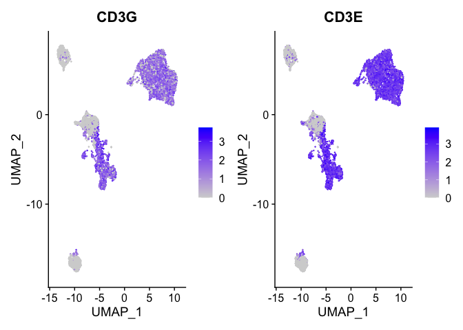
b_cell_markers <- c("CD3G", "CD3E")
FeaturePlot(experiment.aggregate, features = b_cell_markers)
```
```r
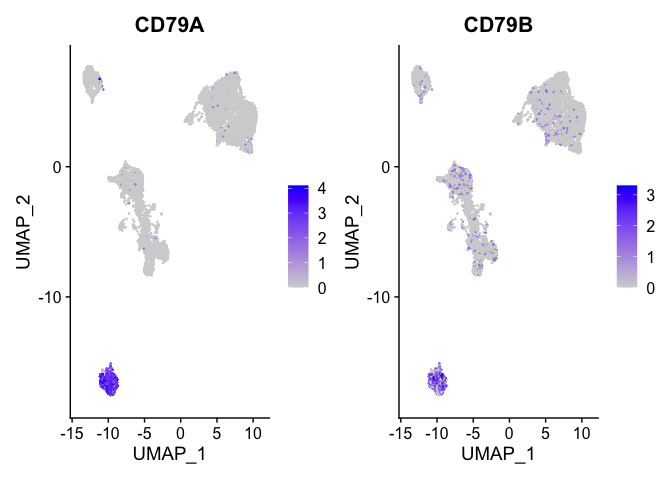
b_cell_markers <- c("CD79A","CD79B")
FeaturePlot(experiment.aggregate, features = b_cell_markers)
```
```r
table(!is.na(experiment.aggregate$CTgene),experiment.aggregate$RNA_snn_res.0.75)
```
0 1 2 3 4 5 6 7 8 9 10 11 12 13
FALSE 2025 1009 959 820 792 643 26 606 513 501 382 282 165 153
TRUE 4 3 3 1 2 9 618 0 4 0 2 1 1 2
14 15 16 17 18 19
FALSE 125 76 2 43 39 19
TRUE 0 1 56 1 0 1
```r
b_cells <- c("6","16")
table(experiment.aggregate$cloneType,experiment.aggregate$RNA_snn_res.0.75)
```
0 1 2 3 4 5 6 7 8 9 10 11 12 13
Single (0 < X <= 1) 3 3 3 1 2 6 565 0 3 0 2 1 1 1
Small (1 < X <= 5) 1 0 0 0 0 3 53 0 1 0 0 0 0 1
14 15 16 17 18 19
Single (0 < X <= 1) 0 1 48 1 0 1
Small (1 < X <= 5) 0 0 8 0 0 0
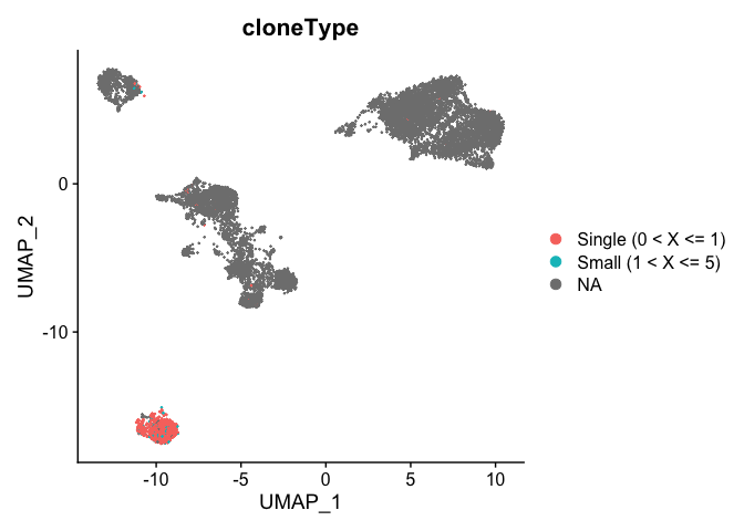
```r
DimPlot(experiment.aggregate, group.by = "cloneType")
```
```r
## find the markers associated with the Clonotypes that contain IGHV1
experiment.aggregate$cells_of_interest <- FALSE
experiment.aggregate$cells_of_interest[grep("IGHV1", experiment.aggregate$CTstrict)] <- TRUE
table(experiment.aggregate$cells_of_interest)
```
FALSE TRUE
9752 137
```r
Idents(experiment.aggregate) <- experiment.aggregate$cells_of_interest
DimPlot(experiment.aggregate)
```

```r
FM <-FindMarkers(experiment.aggregate, ident.1 = "TRUE")
```
```r
table <- table(experiment.aggregate$cloneType, Idents(experiment.aggregate))
table[1,] <- table[1,]/sum(table[1,]) #Scaling by the total number of peripheral B cells
table[2,] <- table[2,]/sum(table[2,]) #Scaling by the total number of tumor B cells
table <- as.data.frame(table)
ggplot(table, aes(x=Var2, y=Freq, fill=Var1)) +
geom_bar(stat="identity", position="fill", color="black", lwd=0.25) +
theme(axis.title.x = element_blank()) +
scale_fill_manual(values = c("#FF4B20","#0348A6")) +
theme_classic() +
theme(axis.title = element_blank()) +
guides(fill=FALSE)
```

```r
experiment.aggregate$cloneType <- factor(experiment.aggregate$cloneType,
levels = c("Hyperexpanded (100 < X <= 500)", "Large (20 < X <= 100)",
"Medium (5 < X <= 20)", "Small (1 < X <= 5)",
"Single (0 < X <= 1)", NA))
DimPlot(experiment.aggregate, group.by = "cloneType")
```

```r
seurat <- highlightClonotypes(experiment.aggregate, cloneCall= "aa",
sequence = c("CARGPSLLWFGEEGYW_CQQANSFPLTF", "NA_CGTWDSGLSGLVF"))
DimPlot(seurat, group.by = "highlight")
```

```r
occupiedscRepertoire(experiment.aggregate, x.axis = "cluster")
```

```r
circles <- getCirclize(experiment.aggregate, cloneCall = "gene+nt", groupBy = "orig.ident" )
```
Using orig.ident as value column: use value.var to override.
Aggregation function missing: defaulting to length
```r
#Just assigning the normal colors to each cluster
grid.cols <- hue_pal()(length(unique(seurat$orig.ident)))
names(grid.cols) <- levels(seurat$orig.ident)
#Graphing the chord diagram
chordDiagram(circles, self.link = 1, grid.col = grid.cols)
```

```r
data_to_circlize <- experiment.aggregate[[]][experiment.aggregate$RNA_snn_res.0.75 %in% b_cells & !is.na(experiment.aggregate$CTgene),]
dim(data_to_circlize)
```
[1] 674 24
```r
head(data_to_circlize)
```
orig.ident nCount_RNA nFeature_RNA percent.mito
AAACCTGTCGCAAGCC-T021PBMC T021PBMC 4086 1377 2.594224
AAAGATGTCCCAAGAT-T021PBMC T021PBMC 3491 1135 4.382698
AAAGTAGTCATCACCC-T021PBMC T021PBMC 7331 1996 3.764834
AAAGTAGTCTGGCGTG-T021PBMC T021PBMC 10667 2809 3.103028
AACCATGGTGCTTCTC-T021PBMC T021PBMC 4084 1474 5.215475
AACCGCGAGAGGGATA-T021PBMC T021PBMC 4478 1491 6.744082
S.Score G2M.Score Phase RNA_snn_res.0.25
AAACCTGTCGCAAGCC-T021PBMC 0.00384910 0.0302408154 G2M 5
AAAGATGTCCCAAGAT-T021PBMC 0.02390299 -0.0436954691 S 5
AAAGTAGTCATCACCC-T021PBMC -0.01221196 -0.0137312346 G1 11
AAAGTAGTCTGGCGTG-T021PBMC -0.03463635 -0.0281840511 G1 11
AACCATGGTGCTTCTC-T021PBMC -0.07459431 -0.0548292439 G1 5
AACCGCGAGAGGGATA-T021PBMC -0.01489864 -0.0009062739 G1 5
RNA_snn_res.0.75 RNA_snn_res.1.25 RNA_snn_res.1.75
AAACCTGTCGCAAGCC-T021PBMC 6 5 7
AAAGATGTCCCAAGAT-T021PBMC 6 5 7
AAAGTAGTCATCACCC-T021PBMC 16 21 24
AAAGTAGTCTGGCGTG-T021PBMC 16 21 24
AACCATGGTGCTTCTC-T021PBMC 6 5 7
AACCGCGAGAGGGATA-T021PBMC 6 5 7
RNA_snn_res.2.25 RNA_snn_res.2.75 RNA_snn_res.3.25
AAACCTGTCGCAAGCC-T021PBMC 6 6 6
AAAGATGTCCCAAGAT-T021PBMC 6 6 6
AAAGTAGTCATCACCC-T021PBMC 26 28 30
AAAGTAGTCTGGCGTG-T021PBMC 26 28 30
AACCATGGTGCTTCTC-T021PBMC 6 6 6
AACCGCGAGAGGGATA-T021PBMC 6 6 6
RNA_snn_res.3.75 seurat_clusters
AAACCTGTCGCAAGCC-T021PBMC 5 5
AAAGATGTCCCAAGAT-T021PBMC 5 5
AAAGTAGTCATCACCC-T021PBMC 33 33
AAAGTAGTCTGGCGTG-T021PBMC 33 33
AACCATGGTGCTTCTC-T021PBMC 5 5
AACCGCGAGAGGGATA-T021PBMC 5 5
barcode
AAACCTGTCGCAAGCC-T021PBMC AAACCTGTCGCAAGCC-T021PBMC
AAAGATGTCCCAAGAT-T021PBMC AAAGATGTCCCAAGAT-T021PBMC
AAAGTAGTCATCACCC-T021PBMC AAAGTAGTCATCACCC-T021PBMC
AAAGTAGTCTGGCGTG-T021PBMC AAAGTAGTCTGGCGTG-T021PBMC
AACCATGGTGCTTCTC-T021PBMC AACCATGGTGCTTCTC-T021PBMC
AACCGCGAGAGGGATA-T021PBMC AACCGCGAGAGGGATA-T021PBMC
CTgene
AAACCTGTCGCAAGCC-T021PBMC IGHV3-30.IGHJ4.IGHD6-13.IGHM_IGLV1-47.IGLJ2.IGLC2
AAAGATGTCCCAAGAT-T021PBMC IGHV1-69D.IGHJ3.IGHD2-2.IGHM_IGLV1-47.IGLJ2.IGLC2
AAAGTAGTCATCACCC-T021PBMC IGHV4-4.IGHJ4.IGHD3-16.IGHM_NA
AAAGTAGTCTGGCGTG-T021PBMC IGHV1-18.IGHJ1..IGHG1_IGKV2D-40.IGKJ2.IGKC
AACCATGGTGCTTCTC-T021PBMC IGHV4-34.IGHJ3.IGHD6-6.IGHM_NA
AACCGCGAGAGGGATA-T021PBMC IGHV3-48.IGHJ6..IGHM_IGLV3-1.IGLJ2.IGLC2
CTnt
AAACCTGTCGCAAGCC-T021PBMC TGTGCGAAAGATTGGGGTATAGCAGCAGCTGGTCCTGATGACTACTGG_TGTGCAGCATGGGATGACAGCCTGAGTGGCGTGGTATTC
AAAGATGTCCCAAGAT-T021PBMC TGTGCGAGTGGGTCCCCCGGAGGATATTGTAGTAGTACCAGCTGCGCTGCTACTGACGCTTTTGATATCTGG_TGTGCAGCATGGGATGACAGCCTGAGTGGTGTGGTATTC
AAAGTAGTCATCACCC-T021PBMC TGTGCGAGAAGACCCGGTGATTACGTTTGGGGGAGTTCATACTGG_TGCATGCAAGCTCTACAAACTCCTCCCACTTTC
AAAGTAGTCTGGCGTG-T021PBMC TGCGCGAGAGGTGGTGCAGCGTACCCCGCTGAATACTTCCAACACTGG_TGCATGCAACGATTAGAGTTTCCTCGGACTTTT
AACCATGGTGCTTCTC-T021PBMC TGTGCGAGAGGCTCTCCGGGTATAGCAGCTCGTCGGGGTGCTTTTGATATCTGG_TGTCAACAGTATTATAGTTTCCCGTACACTTTT
AACCGCGAGAGGGATA-T021PBMC TGTGCGAGAGATTTGTCTATCGGGTACATGGACGTCTGG_TGTCAGGCGTGGGACAGCAGCACTTATGTGGTATTC
CTaa
AAACCTGTCGCAAGCC-T021PBMC CAKDWGIAAAGPDDYW_CAAWDDSLSGVVF
AAAGATGTCCCAAGAT-T021PBMC CASGSPGGYCSSTSCAATDAFDIW_CAAWDDSLSGVVF
AAAGTAGTCATCACCC-T021PBMC CARRPGDYVWGSSYW_CMQALQTPPTF
AAAGTAGTCTGGCGTG-T021PBMC CARGGAAYPAEYFQHW_CMQRLEFPRTF
AACCATGGTGCTTCTC-T021PBMC CARGSPGIAARRGAFDIW_CQQYYSFPYTF
AACCGCGAGAGGGATA-T021PBMC CARDLSIGYMDVW_CQAWDSSTYVVF
CTstrict Frequency
AAACCTGTCGCAAGCC-T021PBMC IGH.2_IGHV3-30_IGLC.2_IGLV1-47 1
AAAGATGTCCCAAGAT-T021PBMC IGH.719_IGHV1-69D_IGLC.595_IGLV1-47 1
AAAGTAGTCATCACCC-T021PBMC IGH.8_IGHV4-4_IGLC.8_IGKV2D-28 1
AAAGTAGTCTGGCGTG-T021PBMC IGH.9_IGHV1-18_IGLC.9_IGKV2D-40 1
AACCATGGTGCTTCTC-T021PBMC IGH.11_IGHV4-34_IGLC.12_IGKV1D-8 1
AACCGCGAGAGGGATA-T021PBMC IGH.12_IGHV3-48_IGLC.13_IGLV3-1 1
cloneType cells_of_interest
AAACCTGTCGCAAGCC-T021PBMC Single (0 < X <= 1) FALSE
AAAGATGTCCCAAGAT-T021PBMC Single (0 < X <= 1) TRUE
AAAGTAGTCATCACCC-T021PBMC Single (0 < X <= 1) FALSE
AAAGTAGTCTGGCGTG-T021PBMC Single (0 < X <= 1) TRUE
AACCATGGTGCTTCTC-T021PBMC Single (0 < X <= 1) FALSE
AACCGCGAGAGGGATA-T021PBMC Single (0 < X <= 1) FALSE
```r
aa_seqs <- strsplit(as.character(unlist(data_to_circlize$CTaa)),split="_")
table(sapply(aa_seqs, length))
```
2
674
```r
data_to_circlize$A_chain = sapply(aa_seqs, "[[", 1L)
data_to_circlize$B_chain = sapply(aa_seqs, "[[", 2L)
data_to_circlize$IGH = sapply(strsplit(data_to_circlize$CTstrict, split="_"), function(x) paste(unique(x[c(1)]),collapse="_"))
data_to_circlize$IGL = sapply(strsplit(data_to_circlize$CTstrict, split="_"), function(x) paste(unique(x[c(3)]),collapse="_"))
# get optimal sequence order from trivial plot
chordDiagram(data.frame(data_to_circlize$IGH[1:15], data_to_circlize$IGL[1:15], times = 1), annotationTrack = "grid" )
```

```r
seq.order <- get.all.sector.index()
circos.clear()
#Phylogenetic tree of B cell evolution
```
## Session Information
```r
sessionInfo()
```
R version 4.0.3 (2020-10-10)
Platform: x86_64-apple-darwin17.0 (64-bit)
Running under: macOS Big Sur 10.16
Matrix products: default
BLAS: /Library/Frameworks/R.framework/Versions/4.0/Resources/lib/libRblas.dylib
LAPACK: /Library/Frameworks/R.framework/Versions/4.0/Resources/lib/libRlapack.dylib
locale:
[1] en_US.UTF-8/en_US.UTF-8/en_US.UTF-8/C/en_US.UTF-8/en_US.UTF-8
attached base packages:
[1] stats graphics grDevices utils datasets methods base
other attached packages:
[1] scRepertoire_1.1.2 scales_1.1.1 circlize_0.4.12 dplyr_1.0.5
[5] cowplot_1.1.1 kableExtra_1.3.4 knitr_1.31 ggplot2_3.3.3
[9] SeuratObject_4.0.0 Seurat_4.0.1
loaded via a namespace (and not attached):
[1] VGAM_1.1-5 systemfonts_1.0.1
[3] plyr_1.8.6 igraph_1.2.6
[5] lazyeval_0.2.2 splines_4.0.3
[7] powerTCR_1.10.3 listenv_0.8.0
[9] scattermore_0.7 GenomeInfoDb_1.24.2
[11] digest_0.6.27 foreach_1.5.1
[13] htmltools_0.5.1.1 ggalluvial_0.12.3
[15] fansi_0.4.2 truncdist_1.0-2
[17] magrittr_2.0.1 doParallel_1.0.16
[19] tensor_1.5 cluster_2.1.1
[21] ROCR_1.0-11 limma_3.44.3
[23] globals_0.14.0 Biostrings_2.56.0
[25] matrixStats_0.58.0 svglite_2.0.0
[27] spatstat.sparse_2.0-0 colorspace_2.0-0
[29] rvest_1.0.0 ggrepel_0.9.1
[31] xfun_0.22 crayon_1.4.1
[33] RCurl_1.98-1.3 jsonlite_1.7.2
[35] spatstat.data_2.1-0 iterators_1.0.13
[37] survival_3.2-10 zoo_1.8-9
[39] glue_1.4.2 polyclip_1.10-0
[41] gtable_0.3.0 zlibbioc_1.34.0
[43] XVector_0.28.0 webshot_0.5.2
[45] leiden_0.3.7 DelayedArray_0.14.1
[47] evd_2.3-3 future.apply_1.7.0
[49] shape_1.4.5 BiocGenerics_0.34.0
[51] SparseM_1.81 abind_1.4-5
[53] DBI_1.1.1 miniUI_0.1.1.1
[55] Rcpp_1.0.6 viridisLite_0.3.0
[57] xtable_1.8-4 reticulate_1.18
[59] spatstat.core_2.0-0 bit_4.0.4
[61] stats4_4.0.3 htmlwidgets_1.5.3
[63] httr_1.4.2 RColorBrewer_1.1-2
[65] ellipsis_0.3.1 ica_1.0-2
[67] farver_2.1.0 pkgconfig_2.0.3
[69] sass_0.3.1 uwot_0.1.10
[71] deldir_0.2-10 utf8_1.2.1
[73] labeling_0.4.2 tidyselect_1.1.0
[75] rlang_0.4.10 reshape2_1.4.4
[77] later_1.1.0.1 munsell_0.5.0
[79] tools_4.0.3 generics_0.1.0
[81] ggridges_0.5.3 evaluate_0.14
[83] stringr_1.4.0 fastmap_1.1.0
[85] yaml_2.2.1 goftest_1.2-2
[87] evmix_2.12 bit64_4.0.5
[89] fitdistrplus_1.1-3 purrr_0.3.4
[91] RANN_2.6.1 pbapply_1.4-3
[93] future_1.21.0 nlme_3.1-152
[95] mime_0.10 xml2_1.3.2
[97] hdf5r_1.3.3 compiler_4.0.3
[99] rstudioapi_0.13 plotly_4.9.3
[101] png_0.1-7 spatstat.utils_2.1-0
[103] tibble_3.1.0 gsl_2.1-6
[105] bslib_0.2.4 stringi_1.5.3
[107] highr_0.8 RSpectra_0.16-0
[109] cubature_2.0.4.1 lattice_0.20-41
[111] Matrix_1.3-2 permute_0.9-5
[113] vegan_2.5-7 vctrs_0.3.6
[115] pillar_1.5.1 lifecycle_1.0.0
[117] spatstat.geom_2.0-1 lmtest_0.9-38
[119] jquerylib_0.1.3 GlobalOptions_0.1.2
[121] RcppAnnoy_0.0.18 data.table_1.14.0
[123] bitops_1.0-6 irlba_2.3.3
[125] httpuv_1.5.5 patchwork_1.1.1
[127] GenomicRanges_1.40.0 R6_2.5.0
[129] promises_1.2.0.1 KernSmooth_2.23-18
[131] gridExtra_2.3 IRanges_2.22.2
[133] parallelly_1.24.0 codetools_0.2-18
[135] MASS_7.3-53.1 assertthat_0.2.1
[137] SummarizedExperiment_1.18.2 withr_2.4.1
[139] sctransform_0.3.2 S4Vectors_0.26.1
[141] GenomeInfoDbData_1.2.3 mgcv_1.8-34
[143] parallel_4.0.3 grid_4.0.3
[145] rpart_4.1-15 tidyr_1.1.3
[147] rmarkdown_2.7 Rtsne_0.15
[149] Biobase_2.48.0 shiny_1.6.0


