
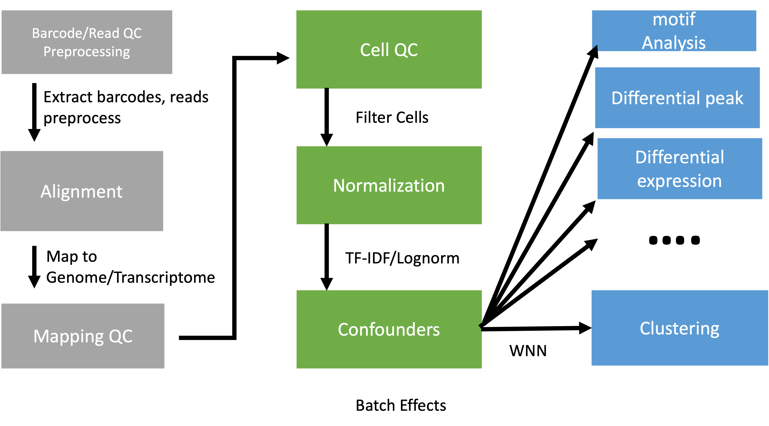
Introduction
There are two types of single cell multiome (considering only gene expression and ATAC) experiments. One is to use single cell multiome kit from 10X and generate gene expression and ATAC libraries from the same cell. The other is to generate gene expression and ATAC libraries from different but same type of cells. The way to analyze these two types of multiome is different. We will start by looking at the experiments where the two sets of libraries are generated from the same cell. Then we will look at the second scenario. Both scenarios require that the scRNASeq data and scATACSeq data are qced separately first.
Install R packages and load the them for importing data to Seurat for QC
if (!requireNamespace("BiocManager", quietly = TRUE)){
    install.packages("BiocManager")
}

if (!requireNamespace("Seurat", quietly = TRUE)){
    install.packages("Seurat")
}

if (!requireNamespace("Signac", quietly = TRUE)){
    BiocManager::install("Signac")
}

if (!requireNamespace("devtools", quietly = TRUE)){
    install.packages("devtools")
}


if (!requireNamespace("SeuratData", quietly = TRUE)){
    devtools::install_github("satijalab/seurat-data")
}

if (!requireNamespace("SoupX", quietly = TRUE)){
    install.packages("SoupX")
}

if (!requireNamespace("DoubletFinder", quietly = TRUE)){
    devtools::install_github("chris-mcginnis-ucsf/DoubletFinder")
}

if (!requireNamespace("AnnotationHub", quietly = TRUE)){
    BiocManager::install("AnnotationHub")
}

if (!requireNamespace("biovizBase", quietly = TRUE)){
    BiocManager::install("biovizBase")
}

if (!requireNamespace("HGNChelper", quietly = TRUE)){
    BiocManager::install("HGNChelper")
}

if (!requireNamespace("kableExtra", quietly = TRUE)){
    install.packages("kableExtra")
}

if (!requireNamespace("BSgenome.Hsapiens.UCSC.hg38", quietly = TRUE)){
    BiocManager::install("BSgenome.Hsapiens.UCSC.hg38")
}


## for motif analysis
if (!requireNamespace("chromVAR", quietly = TRUE)){
    BiocManager::install("chromVAR")
}


if (!requireNamespace("JASPAR2020", quietly = TRUE)){
    BiocManager::install("JASPAR2020")
}

## for transcription factors analysis
if (!requireNamespace("TFBSTools", quietly = TRUE)){
    BiocManager::install("TFBSTools")
}
library(Seurat)
library(DoubletFinder)
library(ggplot2)
Processing scRNASeq and scATAC data separately
Read in cellranger output.
d10x <- Read10X_h5("cellranger_outs/filtered_feature_bc_matrix.h5")
scRNASeq data processing
Read in scRNASeq data
experiment.rna <- CreateSeuratObject(
	d10x$`Gene Expression`,
	min.cells = 0,
	min.features = 0)
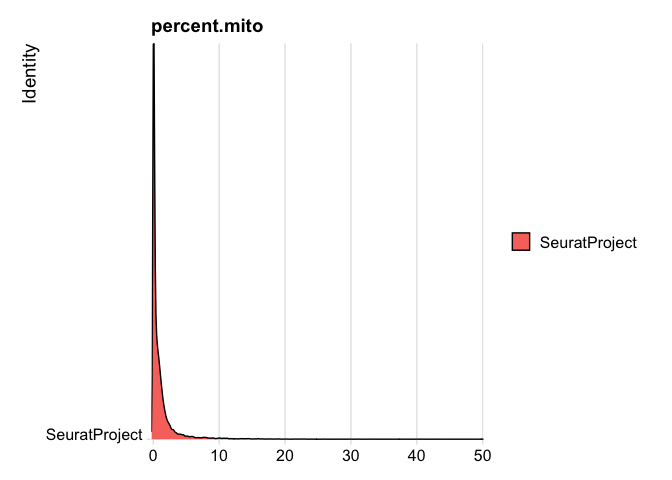
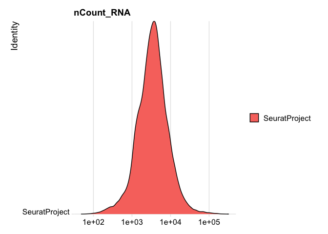
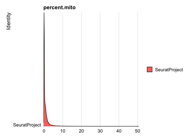
Create some QC metrics and plot
experiment.rna$percent.mito <- PercentageFeatureSet(experiment.rna, pattern = "^MT-")
RidgePlot(experiment.rna, features="percent.mito")
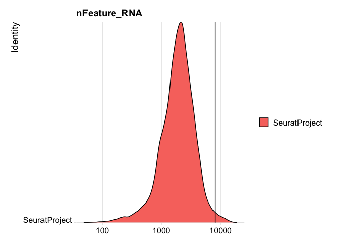
RidgePlot(experiment.rna, features="nFeature_RNA", log=TRUE)

RidgePlot(experiment.rna, features="nCount_RNA", log=TRUE)
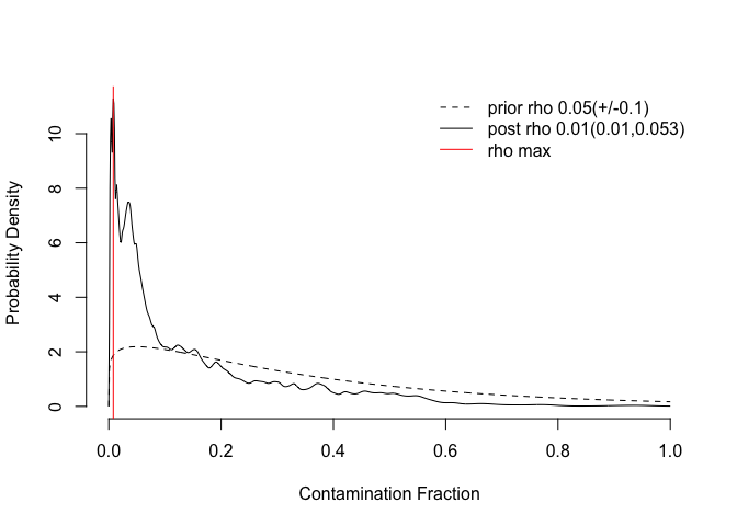
Ambient RNA removal
library(SoupX)
dat <- Read10X_h5("cellranger_outs/raw_feature_bc_matrix.h5")$`Gene Expression`
datCells <- d10x$`Gene Expression`
dat <- dat[rownames(dat),]
clusters <- read.csv("cellranger_outs/analysis/clustering/gex/graphclust/clusters.csv")
mDat <- data.frame(clusters = clusters$Cluster, row.names = clusters$Barcode)
tsne <- read.csv("cellranger_outs/analysis/dimensionality_reduction/gex/tsne_projection.csv")
mDat$tSNE1 <- tsne$TSNE.1[match(rownames(mDat), tsne$Barcode)]
mDat$tSNE2 <- tsne$TSNE.2[match(rownames(mDat), tsne$Barcode)]
DR <- c("tSNE1", "tSNE2")
scdata <- SoupChannel(dat, datCells, mDat)
scdata <- autoEstCont(scdata)
sccounts <- adjustCounts(scdata)
experiment.rna <- CreateSeuratObject(sccounts,
	min.cells = 0,
	min.features = 0)
experiment.rna$percent.mito <- PercentageFeatureSet(experiment.rna, pattern = "^MT-")
RidgePlot(experiment.rna, features="percent.mito")
RidgePlot(experiment.rna, features="nFeature_RNA", log=TRUE) + geom_vline(xintercept = 8000)
RidgePlot(experiment.rna, features="nCount_RNA", log=TRUE) + geom_vline(xintercept = 15000)

Doublet removal
experiment.rna <- subset(experiment.rna, nFeature_RNA >= 500 & nFeature_RNA <= 8000)
experiment.rna <- subset(experiment.rna, nCount_RNA >= 1000 & nCount_RNA <= 12000)
experiment.rna <- NormalizeData(experiment.rna, normalization.method = "LogNormalize", scale.factor = 10000)
experiment.rna <- FindVariableFeatures(experiment.rna, selection.method = "vst", nfeatures = 2000)
experiment.rna <- ScaleData(experiment.rna)
experiment.rna <- RunPCA(experiment.rna)
sweep.res <- paramSweep(experiment.rna, PCs = 1:20, sct = FALSE)
## [1] "Creating artificial doublets for pN = 5%"
## [1] "Creating Seurat object..."
## [1] "Normalizing Seurat object..."
## [1] "Finding variable genes..."
## [1] "Scaling data..."
## [1] "Running PCA..."
## [1] "Calculating PC distance matrix..."
## [1] "Defining neighborhoods..."
## [1] "Computing pANN across all pK..."
## [1] "pK = 5e-04..."
## [1] "pK = 0.001..."
## [1] "pK = 0.005..."
## [1] "pK = 0.01..."
## [1] "pK = 0.02..."
## [1] "pK = 0.03..."
## [1] "pK = 0.04..."
## [1] "pK = 0.05..."
## [1] "pK = 0.06..."
## [1] "pK = 0.07..."
## [1] "pK = 0.08..."
## [1] "pK = 0.09..."
## [1] "pK = 0.1..."
## [1] "pK = 0.11..."
## [1] "pK = 0.12..."
## [1] "pK = 0.13..."
## [1] "pK = 0.14..."
## [1] "pK = 0.15..."
## [1] "pK = 0.16..."
## [1] "pK = 0.17..."
## [1] "pK = 0.18..."
## [1] "pK = 0.19..."
## [1] "pK = 0.2..."
## [1] "pK = 0.21..."
## [1] "pK = 0.22..."
## [1] "pK = 0.23..."
## [1] "pK = 0.24..."
## [1] "pK = 0.25..."
## [1] "pK = 0.26..."
## [1] "pK = 0.27..."
## [1] "pK = 0.28..."
## [1] "pK = 0.29..."
## [1] "pK = 0.3..."
## [1] "Creating artificial doublets for pN = 10%"
## [1] "Creating Seurat object..."
## [1] "Normalizing Seurat object..."
## [1] "Finding variable genes..."
## [1] "Scaling data..."
## [1] "Running PCA..."
## [1] "Calculating PC distance matrix..."
## [1] "Defining neighborhoods..."
## [1] "Computing pANN across all pK..."
## [1] "pK = 5e-04..."
## [1] "pK = 0.001..."
## [1] "pK = 0.005..."
## [1] "pK = 0.01..."
## [1] "pK = 0.02..."
## [1] "pK = 0.03..."
## [1] "pK = 0.04..."
## [1] "pK = 0.05..."
## [1] "pK = 0.06..."
## [1] "pK = 0.07..."
## [1] "pK = 0.08..."
## [1] "pK = 0.09..."
## [1] "pK = 0.1..."
## [1] "pK = 0.11..."
## [1] "pK = 0.12..."
## [1] "pK = 0.13..."
## [1] "pK = 0.14..."
## [1] "pK = 0.15..."
## [1] "pK = 0.16..."
## [1] "pK = 0.17..."
## [1] "pK = 0.18..."
## [1] "pK = 0.19..."
## [1] "pK = 0.2..."
## [1] "pK = 0.21..."
## [1] "pK = 0.22..."
## [1] "pK = 0.23..."
## [1] "pK = 0.24..."
## [1] "pK = 0.25..."
## [1] "pK = 0.26..."
## [1] "pK = 0.27..."
## [1] "pK = 0.28..."
## [1] "pK = 0.29..."
## [1] "pK = 0.3..."
## [1] "Creating artificial doublets for pN = 15%"
## [1] "Creating Seurat object..."
## [1] "Normalizing Seurat object..."
## [1] "Finding variable genes..."
## [1] "Scaling data..."
## [1] "Running PCA..."
## [1] "Calculating PC distance matrix..."
## [1] "Defining neighborhoods..."
## [1] "Computing pANN across all pK..."
## [1] "pK = 5e-04..."
## [1] "pK = 0.001..."
## [1] "pK = 0.005..."
## [1] "pK = 0.01..."
## [1] "pK = 0.02..."
## [1] "pK = 0.03..."
## [1] "pK = 0.04..."
## [1] "pK = 0.05..."
## [1] "pK = 0.06..."
## [1] "pK = 0.07..."
## [1] "pK = 0.08..."
## [1] "pK = 0.09..."
## [1] "pK = 0.1..."
## [1] "pK = 0.11..."
## [1] "pK = 0.12..."
## [1] "pK = 0.13..."
## [1] "pK = 0.14..."
## [1] "pK = 0.15..."
## [1] "pK = 0.16..."
## [1] "pK = 0.17..."
## [1] "pK = 0.18..."
## [1] "pK = 0.19..."
## [1] "pK = 0.2..."
## [1] "pK = 0.21..."
## [1] "pK = 0.22..."
## [1] "pK = 0.23..."
## [1] "pK = 0.24..."
## [1] "pK = 0.25..."
## [1] "pK = 0.26..."
## [1] "pK = 0.27..."
## [1] "pK = 0.28..."
## [1] "pK = 0.29..."
## [1] "pK = 0.3..."
## [1] "Creating artificial doublets for pN = 20%"
## [1] "Creating Seurat object..."
## [1] "Normalizing Seurat object..."
## [1] "Finding variable genes..."
## [1] "Scaling data..."
## [1] "Running PCA..."
## [1] "Calculating PC distance matrix..."
## [1] "Defining neighborhoods..."
## [1] "Computing pANN across all pK..."
## [1] "pK = 5e-04..."
## [1] "pK = 0.001..."
## [1] "pK = 0.005..."
## [1] "pK = 0.01..."
## [1] "pK = 0.02..."
## [1] "pK = 0.03..."
## [1] "pK = 0.04..."
## [1] "pK = 0.05..."
## [1] "pK = 0.06..."
## [1] "pK = 0.07..."
## [1] "pK = 0.08..."
## [1] "pK = 0.09..."
## [1] "pK = 0.1..."
## [1] "pK = 0.11..."
## [1] "pK = 0.12..."
## [1] "pK = 0.13..."
## [1] "pK = 0.14..."
## [1] "pK = 0.15..."
## [1] "pK = 0.16..."
## [1] "pK = 0.17..."
## [1] "pK = 0.18..."
## [1] "pK = 0.19..."
## [1] "pK = 0.2..."
## [1] "pK = 0.21..."
## [1] "pK = 0.22..."
## [1] "pK = 0.23..."
## [1] "pK = 0.24..."
## [1] "pK = 0.25..."
## [1] "pK = 0.26..."
## [1] "pK = 0.27..."
## [1] "pK = 0.28..."
## [1] "pK = 0.29..."
## [1] "pK = 0.3..."
## [1] "Creating artificial doublets for pN = 25%"
## [1] "Creating Seurat object..."
## [1] "Normalizing Seurat object..."
## [1] "Finding variable genes..."
## [1] "Scaling data..."
## [1] "Running PCA..."
## [1] "Calculating PC distance matrix..."
## [1] "Defining neighborhoods..."
## [1] "Computing pANN across all pK..."
## [1] "pK = 5e-04..."
## [1] "pK = 0.001..."
## [1] "pK = 0.005..."
## [1] "pK = 0.01..."
## [1] "pK = 0.02..."
## [1] "pK = 0.03..."
## [1] "pK = 0.04..."
## [1] "pK = 0.05..."
## [1] "pK = 0.06..."
## [1] "pK = 0.07..."
## [1] "pK = 0.08..."
## [1] "pK = 0.09..."
## [1] "pK = 0.1..."
## [1] "pK = 0.11..."
## [1] "pK = 0.12..."
## [1] "pK = 0.13..."
## [1] "pK = 0.14..."
## [1] "pK = 0.15..."
## [1] "pK = 0.16..."
## [1] "pK = 0.17..."
## [1] "pK = 0.18..."
## [1] "pK = 0.19..."
## [1] "pK = 0.2..."
## [1] "pK = 0.21..."
## [1] "pK = 0.22..."
## [1] "pK = 0.23..."
## [1] "pK = 0.24..."
## [1] "pK = 0.25..."
## [1] "pK = 0.26..."
## [1] "pK = 0.27..."
## [1] "pK = 0.28..."
## [1] "pK = 0.29..."
## [1] "pK = 0.3..."
## [1] "Creating artificial doublets for pN = 30%"
## [1] "Creating Seurat object..."
## [1] "Normalizing Seurat object..."
## [1] "Finding variable genes..."
## [1] "Scaling data..."
## [1] "Running PCA..."
## [1] "Calculating PC distance matrix..."
## [1] "Defining neighborhoods..."
## [1] "Computing pANN across all pK..."
## [1] "pK = 5e-04..."
## [1] "pK = 0.001..."
## [1] "pK = 0.005..."
## [1] "pK = 0.01..."
## [1] "pK = 0.02..."
## [1] "pK = 0.03..."
## [1] "pK = 0.04..."
## [1] "pK = 0.05..."
## [1] "pK = 0.06..."
## [1] "pK = 0.07..."
## [1] "pK = 0.08..."
## [1] "pK = 0.09..."
## [1] "pK = 0.1..."
## [1] "pK = 0.11..."
## [1] "pK = 0.12..."
## [1] "pK = 0.13..."
## [1] "pK = 0.14..."
## [1] "pK = 0.15..."
## [1] "pK = 0.16..."
## [1] "pK = 0.17..."
## [1] "pK = 0.18..."
## [1] "pK = 0.19..."
## [1] "pK = 0.2..."
## [1] "pK = 0.21..."
## [1] "pK = 0.22..."
## [1] "pK = 0.23..."
## [1] "pK = 0.24..."
## [1] "pK = 0.25..."
## [1] "pK = 0.26..."
## [1] "pK = 0.27..."
## [1] "pK = 0.28..."
## [1] "pK = 0.29..."
## [1] "pK = 0.3..."
sweep.stats <- summarizeSweep(sweep.res, GT = FALSE)
bcmvn <- find.pK(sweep.stats)
## NULL
pK.set <- bcmvn$pK[which(bcmvn$BCmetric == max(bcmvn$BCmetric))]
nExp_poi <- round(0.08 * nrow(experiment.rna@meta.data))
experiment.rna <- doubletFinder(experiment.rna, PCs = 1:20, pN = 0.25, pK = as.numeric(as.character(pK.set)), nExp = nExp_poi, reuse.pANN = FALSE, sct = FALSE)
## [1] "Creating 6440 artificial doublets..."
## [1] "Creating Seurat object..."
## [1] "Normalizing Seurat object..."
## [1] "Finding variable genes..."
## [1] "Scaling data..."
## [1] "Running PCA..."
## [1] "Calculating PC distance matrix..."
## [1] "Computing pANN..."
## [1] "Classifying doublets.."
cls <- grep("DF.classifications", names(experiment.rna@meta.data))
counts <- sccounts[, match(colnames(experiment.rna)[experiment.rna@meta.data[cls]=="Singlet"], colnames(sccounts))]
Standard scRNASeq data processing
experiment.aggregate <- CreateSeuratObject(counts)
experiment.aggregate <- NormalizeData(experiment.aggregate, normalization.method = "LogNormalize", scale.factor = 10000)

s.genes <- cc.genes.updated.2019$s.genes
g2m.genes <- cc.genes.updated.2019$g2m.genes

experiment.aggregate <- CellCycleScoring(experiment.aggregate,
                                         s.features = s.genes,
                                         g2m.features = g2m.genes,
                                         set.ident = TRUE)

experiment.aggregate <- ScaleData(experiment.aggregate,
                                  vars.to.regress = c("S.Score", "G2M.Score", "nFeature_RNA"))

saveRDS(experiment.aggregate, "scrna.rds")
scATACSeq data processing
library(AnnotationHub)
ah <- AnnotationHub()
qr <- query(ah, c("Homo sapiens", "EnsDb", "GRCh38"))
edb <- qr[[1]]
library(Signac)
library(biovizBase)

atac_counts <- d10x$Peaks
grange.counts <- StringToGRanges(rownames(atac_counts), sep=c(":", "-"))
grange.use <- seqnames(grange.counts) %in% standardChromosomes(grange.counts)
atac_counts <- atac_counts[as.vector(grange.use),]
annotations <- GetGRangesFromEnsDb(ensdb = edb)
seqlevelsStyle(annotations) <- 'UCSC'
genome(annotations) <- "GRCh38"

atac_assay <- CreateChromatinAssay(
        counts = atac_counts, sep = c(":", "-"), genome = "GRCh38",
        fragments = "./cellranger_outs/atac_fragments.tsv.gz",
        annotation = annotations)

## remove the cells that have been filtered out in scRNA data
experiment.aggregate <- readRDS("scrna.rds")
atac_assay <- subset(atac_assay, cells = colnames(experiment.aggregate))

experiment.atac <- CreateSeuratObject(
	atac_assay,
	assay = "ATAC")
QC metrics and plots
## When individual sample per_barcode_metrics.csv is available, the following metrics can be calculated
#experiment.atac$pct_reads_in_peaks <- experiment.atac$atac_peak_region_fragments / experiment.atac$atac_fragments * 100
## blacklist regions created by ENCODE project
experiment.atac$blacklist_ratio <- FractionCountsInRegion(
object = experiment.atac,
assay = 'ATAC',
regions = blacklist_hg38_unified
)
experiment.atac <- TSSEnrichment(object = experiment.atac, fast = FALSE)
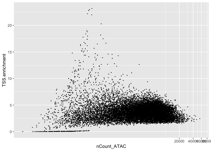
## scatter plot to easily identify filtering criteria
DensityScatter(experiment.atac, x = 'nCount_ATAC', y = 'TSS.enrichment', log_x = T, quantiles = T)
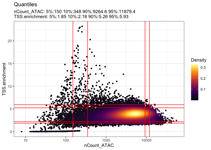
d2p <- data.frame(nCount_ATAC = experiment.atac$nCount_ATAC, TSS.enrichment = experiment.atac$TSS.enrichment)
ggplot(d2p, aes(x = nCount_ATAC, y = TSS.enrichment)) + geom_point(size = 0.1) + coord_trans(x = "log10")
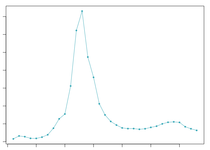
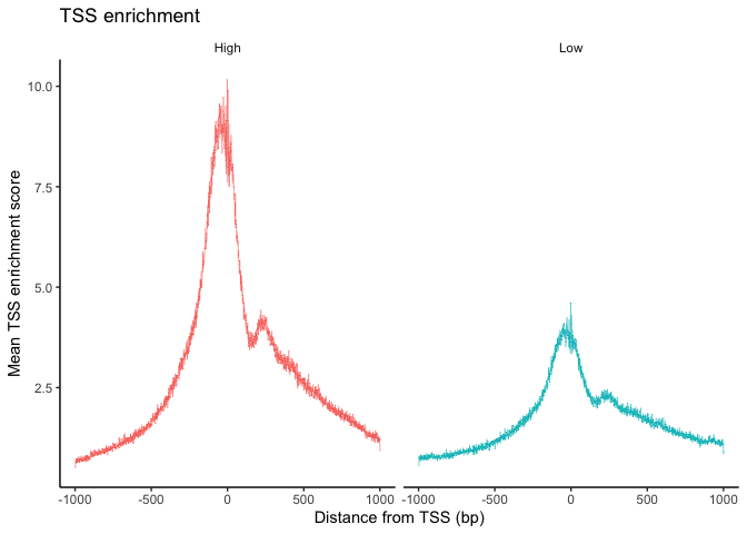
## TSS enrichment plot
experiment.atac$high.tss <- ifelse(experiment.atac$TSS.enrichment > 3, 'High', 'Low')
TSSPlot(experiment.atac, group.by = 'high.tss') + NoLegend()
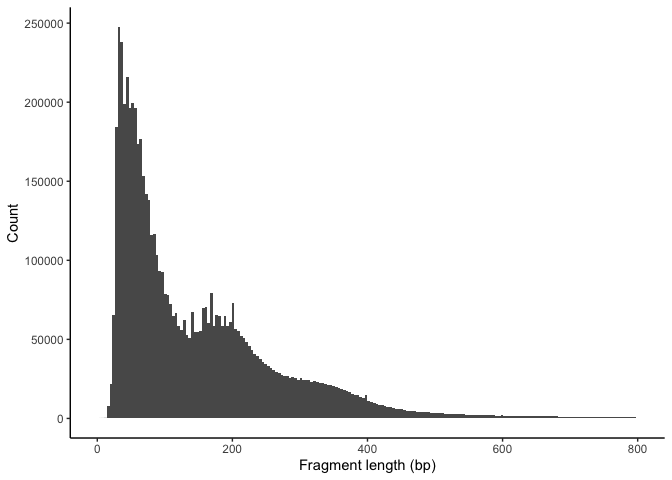
## Nucleosome signal plot
experiment.atac <- NucleosomeSignal(object = experiment.atac, assay = "ATAC")

experiment.atac$nucleosome_group <- ifelse(experiment.atac$nucleosome_signal > 4, 'NS > 4', 'NS <= 4')
FragmentHistogram(object = experiment.atac, assay = "ATAC", group.by = NULL, region = "chr1-1-20000000")
scATAC QC filtering
experiment.atac <- subset(experiment.atac, subset = nCount_ATAC > 2300 & nCount_ATAC < 40000 & blacklist_ratio < 0.05 & nucleosome_signal < 4 & TSS.enrichment > 3)
saveRDS(experiment.atac, "scatac.rds")
Analysis by combining scRNA and scATAC data before clustering
experiment.aggregate <- experiment.aggregate[, colnames(experiment.aggregate) %in% colnames(experiment.atac)]
atac_assay <- subset(atac_assay, cells = colnames(experiment.atac))
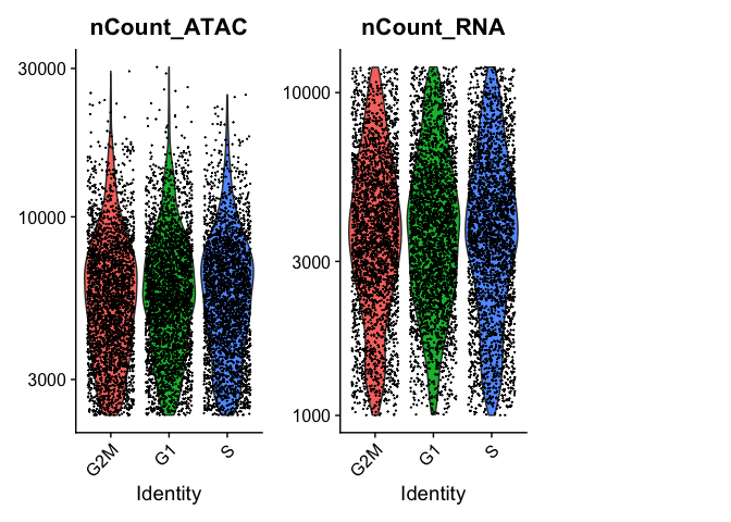
experiment.aggregate[["ATAC"]] <- atac_assay
VlnPlot(experiment.aggregate, features = c("nCount_ATAC", "nCount_RNA"), ncol = 3, log = T)
Performing dimensionality reduction on scRNA and scATAC data
## dimensionality reduction scRNA
DefaultAssay(experiment.aggregate) <- "RNA"
experiment.aggregate <- FindVariableFeatures(experiment.aggregate)
experiment.aggregate <- RunPCA(experiment.aggregate)
experiment.aggregate <- RunUMAP(experiment.aggregate,
                                reduction = "pca", reduction.name = "umap.rna", reduction.key = "rnaUMAP_",
                                dims = 1:30)


## dimensionality reduction scATAC
DefaultAssay(experiment.aggregate) <- "ATAC"
experiment.aggregate <- RunTFIDF(experiment.aggregate)
experiment.aggregate <- FindTopFeatures(experiment.aggregate, min.cutoff = 'q0')
experiment.aggregate <- RunSVD(experiment.aggregate)
experiment.aggregate <- RunUMAP(experiment.aggregate,
                                reduction = 'lsi',
                                dims = 2:50,
                                reduction.name = "umap.atac", reduction.key = "atacUMAP_")
saveRDS(experiment.aggregate, "bimodal.nomalized.rds")
Clustering scRNA and scATAC data together using weighted nearest neighbor analysis
Weighted nearest neighbor analysis was introduced by the Satija Lab in [2021] (https://www.sciencedirect.com/science/article/pii/S0092867421005833?via%3Dihub). It is a framework to integrate multiple data types that are measured within a cell. It uses a unsupervised approach to learn the cell-specific “weights” for each modality, which will be used in downstream analysis. The workflow was designed to be robust to vast differences in data quality between different modalities and enable multiple downstream analyses using this integrated framework, such as visualization, clustering, trajectory analysis. The ultimate goal is to enable better characterization of cell states. The workflow involves four steps:
1. Constructing independent k nearest neighbor graphs for both modalities
2. Performing with and across-modality prediction
3. Calculating cell-specific modality weights
4. Calculating a WNN graph
experiment.aggregate <- readRDS("bimodal.nomalized.rds")
experiment.aggregate <- FindMultiModalNeighbors(experiment.aggregate, reduction.list = list("pca", "lsi"),
dims.list = list(1:30, 2:50))
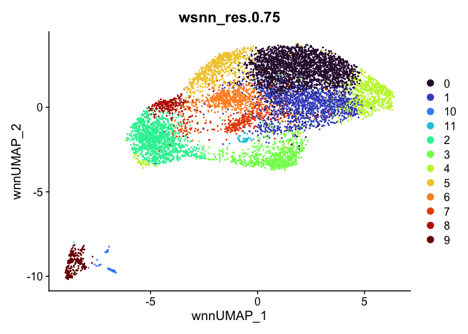
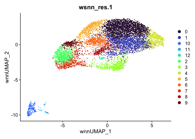
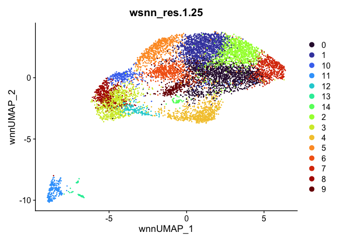
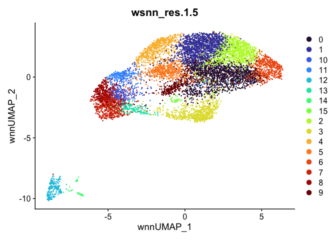
experiment.aggregate <- FindClusters(experiment.aggregate, graph.name = "wsnn", resolution = seq(0.75, 1.5, 0.25), algorithm = 3, verbose = F)
experiment.aggregate <- RunUMAP(experiment.aggregate, nn.name = "weighted.nn",
reduction.name = "umap.wnn", reduction.key = "wnnUMAP_")
Let’s take a look at the clusters.
outputs <- lapply(grep("wsnn", colnames(experiment.aggregate@meta.data), value=TRUE), function(res){
        dimplot <- DimPlot(experiment.aggregate, reduction = "umap.wnn", group.by = res, shuffle = TRUE) +
                scale_color_viridis_d(option = "turbo") + ggtitle(res)
        return(list(dimplot=dimplot))
})
for (i in 1:length(outputs)){
        cat("\n\n\n\n")
        print(outputs[[i]]$dimplot)
        cat("\n\n\n\n")
}
Automatic cell type annotation using scRNA profile.
library(HGNChelper)
library(kableExtra)
source("https://raw.githubusercontent.com/IanevskiAleksandr/sc-type/master/R/gene_sets_prepare.R")
# load cell type annotation function
source("https://raw.githubusercontent.com/IanevskiAleksandr/sc-type/master/R/sctype_score_.R")

db = "https://raw.githubusercontent.com/IanevskiAleksandr/sc-type/master/ScTypeDB_full.xlsx"
tissues = "Kidney"

gs_list <- gene_sets_prepare(db, tissues)

# get the cell type marker genes' data
gene.features <- unique(unlist(c(gs_list)))
#scRNAseqData <- FetchData(experiment.aggregate, assay = "RNA", vars = rownames(experiment.aggregate[["RNA"]]))
scRNAseqData <- FetchData(experiment.aggregate, assay = "RNA", vars = gene.features, layer = "scale.data")
colnames(scRNAseqData) <- sapply(colnames(scRNAseqData), function(x){gsub("rna_", "", x)})
scRNAseqData <- t(scRNAseqData)

## cell type annotation
cy.max <- sctype_score(scRNAseqData, scaled = TRUE, gs = gs_list$gs_positive, gs2 = gs_list$gs_negative)

cC_results <- do.call(rbind, lapply(unique(experiment.aggregate@meta.data$wsnn_res.0.75), function(cluster){
        cy.max.cluster <- sort(rowSums(cy.max[,rownames(experiment.aggregate@meta.data[experiment.aggregate@meta.data$wsnn_res.0.75 == cluster, ])]), decreasing = TRUE)
        head(data.frame(cluster=cluster, type=names(cy.max.cluster), scores=cy.max.cluster, ncells=sum(experiment.aggregate@meta.data$wsnn_res.0.75 == cluster)), 10)
}))

sctype_scores <- cC_results %>% dplyr::group_by(cluster) %>% dplyr::slice_max(n=1, order_by=scores)
kable(sctype_scores[,1:3], caption="Initial Cell type assignment", "html") %>% kable_styling("striped")
| cluster | type | scores |
|---|---|---|
| 0 | Principal cells (Collecting duct system) | 37.37502 |
| 1 | Proximal tubule cells | 194.42203 |
| 10 | Endothelial cells | 276.75519 |
| 11 | Ureteric Bud cells | 11.07892 |
| 2 | Loop of Henle cells | 918.87678 |
| 3 | Mesangial cells | 112.19081 |
| 4 | Proximal tubule cells | 1089.02504 |
| 5 | Cap mesenchyme cells (Mesenchymal cells) | 22.44973 |
| 6 | Podocytes | 74.47326 |
| 7 | Stromal cells | 156.93031 |
| 8 | Loop of Henle cells | 109.95110 |
| 9 | Hematopoietic cells | 803.16847 |
# set low sc-type score clusters to "unknown"
sctype_scores$type[as.numeric(as.character(sctype_scores$scores)) < sctype_scores$ncells/4] <- "Unknown"
kable(sctype_scores[,1:3], caption="Final Cell type assignment", "html") %>% kable_styling("striped")
| cluster | type | scores |
|---|---|---|
| 0 | Unknown | 37.37502 |
| 1 | Unknown | 194.42203 |
| 10 | Endothelial cells | 276.75519 |
| 11 | Unknown | 11.07892 |
| 2 | Loop of Henle cells | 918.87678 |
| 3 | Unknown | 112.19081 |
| 4 | Proximal tubule cells | 1089.02504 |
| 5 | Unknown | 22.44973 |
| 6 | Unknown | 74.47326 |
| 7 | Stromal cells | 156.93031 |
| 8 | Loop of Henle cells | 109.95110 |
| 9 | Hematopoietic cells | 803.16847 |
# label cells with cell type
experiment.aggregate@meta.data$CellType.wsnn_res.0.75 <- ""
for (i in unique(sctype_scores$cluster)){
celltype <- sctype_scores[sctype_scores$cluster == i,]
experiment.aggregate@meta.data$CellType.wsnn_res.0.75[experiment.aggregate@meta.data$wsnn_res.0.75 == i] <- as.character(celltype$type[1])
}
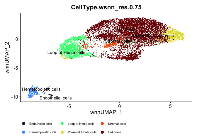
DimPlot(experiment.aggregate, reduction = "umap.wnn", label = TRUE, repel = TRUE, group.by = "CellType.wsnn_res.0.75", shuffle = TRUE) +
scale_color_viridis_d(option = "turbo") + ggplot2::theme(legend.position="bottom", legend.text=element_text(size=8))
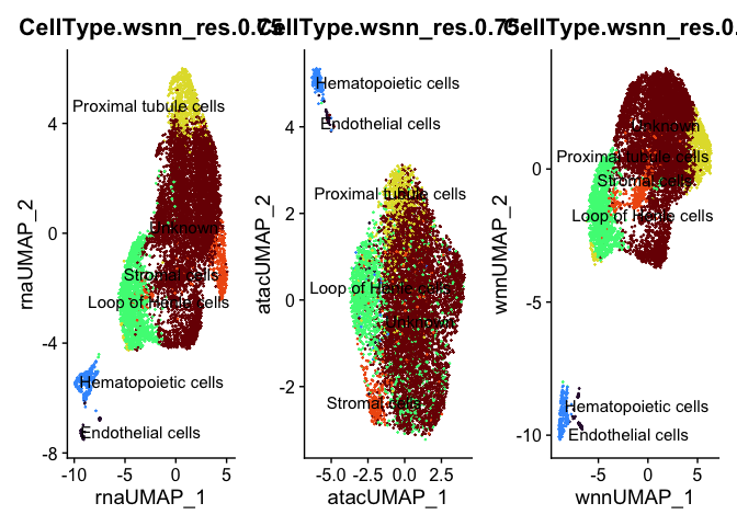
p1 <- DimPlot(experiment.aggregate, reduction = "umap.rna", label = TRUE, repel = TRUE, group.by = "CellType.wsnn_res.0.75", shuffle = TRUE) +
        scale_color_viridis_d(option = "turbo") + NoLegend()


p2 <- DimPlot(experiment.aggregate, reduction = "umap.atac", label = TRUE, repel = TRUE, group.by = "CellType.wsnn_res.0.75", shuffle = TRUE) +
        scale_color_viridis_d(option = "turbo") + NoLegend()

p3 <- DimPlot(experiment.aggregate, reduction = "umap.wnn", label = TRUE, repel = TRUE, group.by = "CellType.wsnn_res.0.75", shuffle = TRUE) +
        scale_color_viridis_d(option = "turbo") + NoLegend()

p1 + p2 + p3
Find markers
Idents(experiment.aggregate) <- "CellType.wsnn_res.0.75"
DefaultAssay(experiment.aggregate) <- "RNA"
gene.markers <- FindMarkers(experiment.aggregate, ident.1 = "Hematopoietic cells", only.pos=FALSE, min.pct=0.25, logfc.threshold=0.25)
kable(gene.markers[1:100,], 'html', align='c') %>% kable_styling() %>% scroll_box(height="500px")
| p_val | avg_log2FC | pct.1 | pct.2 | p_val_adj | |
|---|---|---|---|---|---|
| LDLRAD4 | 0 | 7.442599 | 0.811 | 0.019 | 0 |
| ARHGAP15 | 0 | 6.912135 | 0.758 | 0.011 | 0 |
| CELF2 | 0 | 5.702955 | 0.789 | 0.063 | 0 |
| KCNMA1 | 0 | 6.164893 | 0.775 | 0.067 | 0 |
| PTPRC | 0 | 6.241130 | 0.700 | 0.007 | 0 |
| MSR1 | 0 | 5.408020 | 0.762 | 0.073 | 0 |
| CHST11 | 0 | 5.490887 | 0.753 | 0.067 | 0 |
| TBXAS1 | 0 | 6.251135 | 0.700 | 0.034 | 0 |
| RGS1 | 0 | 9.519696 | 0.652 | 0.004 | 0 |
| PDE4B | 0 | 7.250954 | 0.648 | 0.011 | 0 |
| DOCK2 | 0 | 6.799417 | 0.648 | 0.011 | 0 |
| SLC1A3 | 0 | 11.397819 | 0.617 | 0.001 | 0 |
| LINC00278 | 0 | 9.322655 | 0.595 | 0.002 | 0 |
| CD74 | 0 | 6.448059 | 0.612 | 0.032 | 0 |
| PREX1 | 0 | 8.146827 | 0.581 | 0.003 | 0 |
| MEF2C | 0 | 6.563517 | 0.590 | 0.021 | 0 |
| INPP5D | 0 | 6.262607 | 0.581 | 0.019 | 0 |
| SRGN | 0 | 7.467014 | 0.564 | 0.012 | 0 |
| AOAH | 0 | 5.913373 | 0.568 | 0.023 | 0 |
| CIITA | 0 | 7.265145 | 0.551 | 0.010 | 0 |
| DOCK10 | 0 | 6.387843 | 0.546 | 0.008 | 0 |
| FYB1 | 0 | 7.361728 | 0.542 | 0.006 | 0 |
| FAM49A | 0 | 10.190762 | 0.533 | 0.002 | 0 |
| FKBP5 | 0 | 6.925745 | 0.542 | 0.011 | 0 |
| PIK3R5 | 0 | 8.019027 | 0.533 | 0.003 | 0 |
| GPNMB | 0 | 8.054225 | 0.529 | 0.008 | 0 |
| HLA-DRA | 0 | 6.439959 | 0.537 | 0.019 | 0 |
| UTY | 0 | 7.167129 | 0.502 | 0.004 | 0 |
| MS4A6A | 0 | 10.146818 | 0.489 | 0.001 | 0 |
| ZNF804A | 0 | 9.471391 | 0.489 | 0.003 | 0 |
| SAMSN1 | 0 | 7.210423 | 0.489 | 0.006 | 0 |
| ITGAX | 0 | 9.694704 | 0.480 | 0.002 | 0 |
| PDE3B | 0 | 6.789981 | 0.489 | 0.012 | 0 |
| KYNU | 0 | 9.478806 | 0.458 | 0.002 | 0 |
| L3MBTL4 | 0 | 6.425959 | 0.467 | 0.012 | 0 |
| FLI1 | 0 | 6.657869 | 0.454 | 0.004 | 0 |
| HLA-DPB1 | 0 | 6.458288 | 0.458 | 0.011 | 0 |
| TNFRSF1B | 0 | 7.553422 | 0.427 | 0.003 | 0 |
| IRAK3 | 0 | 9.589055 | 0.423 | 0.002 | 0 |
| MS4A7 | 0 | 8.738475 | 0.419 | 0.002 | 0 |
| CTSS | 0 | 6.250552 | 0.427 | 0.012 | 0 |
| PCED1B | 0 | 6.497238 | 0.419 | 0.007 | 0 |
| LINC01374 | 0 | 8.015152 | 0.410 | 0.004 | 0 |
| ST8SIA4 | 0 | 8.949004 | 0.401 | 0.002 | 0 |
| WDFY4 | 0 | 6.565779 | 0.396 | 0.009 | 0 |
| GAS7 | 0 | 7.346746 | 0.392 | 0.007 | 0 |
| HLA-DPA1 | 0 | 6.435030 | 0.392 | 0.010 | 0 |
| RTN1 | 0 | 6.821210 | 0.388 | 0.008 | 0 |
| CSF2RA | 0 | 8.394648 | 0.379 | 0.002 | 0 |
| LAPTM5 | 0 | 8.221312 | 0.379 | 0.003 | 0 |
| SLA | 0 | 6.567346 | 0.370 | 0.004 | 0 |
| MS4A4E | 0 | 8.817747 | 0.366 | 0.003 | 0 |
| BASP1 | 0 | 7.840451 | 0.366 | 0.004 | 0 |
| OLR1 | 0 | 11.184424 | 0.361 | 0.000 | 0 |
| NRP2 | 0 | 6.434487 | 0.366 | 0.010 | 0 |
| USP9Y | 0 | 6.561384 | 0.357 | 0.005 | 0 |
| IL10RA | 0 | 8.198665 | 0.348 | 0.001 | 0 |
| LCP2 | 0 | 6.538779 | 0.344 | 0.003 | 0 |
| SLC2A3 | 0 | 7.355856 | 0.348 | 0.007 | 0 |
| CD86 | 0 | 9.545345 | 0.339 | 0.001 | 0 |
| PADI2 | 0 | 9.938869 | 0.339 | 0.002 | 0 |
| FCGR2A | 0 | 8.769063 | 0.335 | 0.002 | 0 |
| CXCR4 | 0 | 6.483729 | 0.335 | 0.005 | 0 |
| C1QB | 0 | 6.346739 | 0.335 | 0.009 | 0 |
| SLC11A1 | 0 | 8.262644 | 0.330 | 0.004 | 0 |
| HCLS1 | 0 | 7.064875 | 0.330 | 0.004 | 0 |
| KLHL6 | 0 | 8.440148 | 0.322 | 0.003 | 0 |
| HLA-DQA1 | 0 | 6.924711 | 0.313 | 0.004 | 0 |
| CLEC7A | 0 | 9.390614 | 0.308 | 0.001 | 0 |
| MS4A4A | 0 | 7.887890 | 0.308 | 0.002 | 0 |
| AC079793.1 | 0 | 6.408098 | 0.308 | 0.004 | 0 |
| BCAT1 | 0 | 8.851881 | 0.304 | 0.002 | 0 |
| IKZF1 | 0 | 6.024952 | 0.304 | 0.004 | 0 |
| PECAM1 | 0 | 5.974864 | 0.304 | 0.006 | 0 |
| PALD1 | 0 | 7.607121 | 0.295 | 0.003 | 0 |
| HLA-DMB | 0 | 6.766732 | 0.291 | 0.005 | 0 |
| TRPM2 | 0 | 8.640227 | 0.286 | 0.001 | 0 |
| CSF1R | 0 | 7.629998 | 0.282 | 0.002 | 0 |
| RCSD1 | 0 | 7.598245 | 0.282 | 0.003 | 0 |
| TYROBP | 0 | 7.354642 | 0.282 | 0.004 | 0 |
| C22orf34 | 0 | 6.369845 | 0.278 | 0.003 | 0 |
| PARVG | 0 | 8.695069 | 0.269 | 0.001 | 0 |
| FPR3 | 0 | 8.742942 | 0.264 | 0.001 | 0 |
| CD84 | 0 | 7.591719 | 0.260 | 0.002 | 0 |
| NPL | 0 | 6.017694 | 0.441 | 0.019 | 0 |
| HLA-DQB1 | 0 | 6.259602 | 0.282 | 0.005 | 0 |
| HLA-DRB1 | 0 | 5.706491 | 0.507 | 0.033 | 0 |
| PLAUR | 0 | 6.655959 | 0.282 | 0.007 | 0 |
| GNB4 | 0 | 5.787862 | 0.392 | 0.018 | 0 |
| C3 | 0 | 5.887943 | 0.339 | 0.013 | 0 |
| TCF4 | 0 | 4.841006 | 0.634 | 0.061 | 0 |
| CD14 | 0 | 6.214429 | 0.256 | 0.006 | 0 |
| SLC8A1 | 0 | 4.827451 | 0.855 | 0.129 | 0 |
| TENM4 | 0 | 5.764003 | 0.396 | 0.020 | 0 |
| C1QA | 0 | 6.380802 | 0.269 | 0.007 | 0 |
| APOC1 | 0 | 6.000852 | 0.308 | 0.012 | 0 |
| GLUL | 0 | 5.450771 | 0.423 | 0.025 | 0 |
| RUNX1 | 0 | 4.981378 | 0.590 | 0.055 | 0 |
| TPRG1 | 0 | 5.765792 | 0.476 | 0.034 | 0 |
| CPM | 0 | 6.291475 | 0.427 | 0.027 | 0 |
Some visualizations of scRNA and scATAC data
library(BSgenome.Hsapiens.UCSC.hg38)
library(ggforce)
Idents(experiment.aggregate) <- "CellType.wsnn_res.0.75"
DefaultAssay(experiment.aggregate) <- "ATAC"
experiment.aggregate <- RegionStats(experiment.aggregate, genome = BSgenome.Hsapiens.UCSC.hg38)
#experiment.aggregate <- LinkPeaks(experiment.aggregate, peak.assay = "ATAC", expression.assay = "RNA")
#saveRDS(experiment.aggregate, "linked.rds")
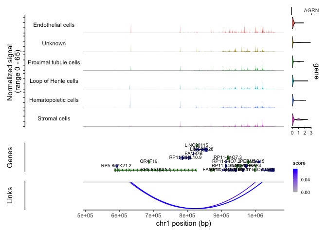
experiment.aggregate <- readRDS("linked.rds")
CoveragePlot(experiment.aggregate, region = "AGRN", features = "AGRN", assay = "ATAC", expression.assay = "RNA", links = TRUE, peaks = FALSE, extend.upstream = 500000, extend.downstream = 2000)
Motif analysis
library(chromVAR)
library(JASPAR2020)
library(TFBSTools)
library(ggseqlogo)
DefaultAssay <- "ATAC"
pfm <- getMatrixSet(x = JASPAR2020, opts = list(species = 9606, all_versions = F))
experiment.aggregate <- AddMotifs(experiment.aggregate, genome = BSgenome.Hsapiens.UCSC.hg38, pfm = pfm)
## Peak markers
Idents(experiment.aggregate) <- "CellType.wsnn_res.0.75"
de.peaks <- FindMarkers(experiment.aggregate, ident.1 = "Proximal tubule cells", ident.2 = unique(experiment.aggregate$CellType.wsnn_res.0.75)[6],
only.pos = T, test.use = 'LR', min.pct = 0.10, latent.vars = "nCount_ATAC")
top.de.peaks <- rownames(de.peaks[de.peaks$p_val < 0.005 & de.peaks$pct.1 > 0.3, ])
## Find enriched motifs in the top differential abundant peaks
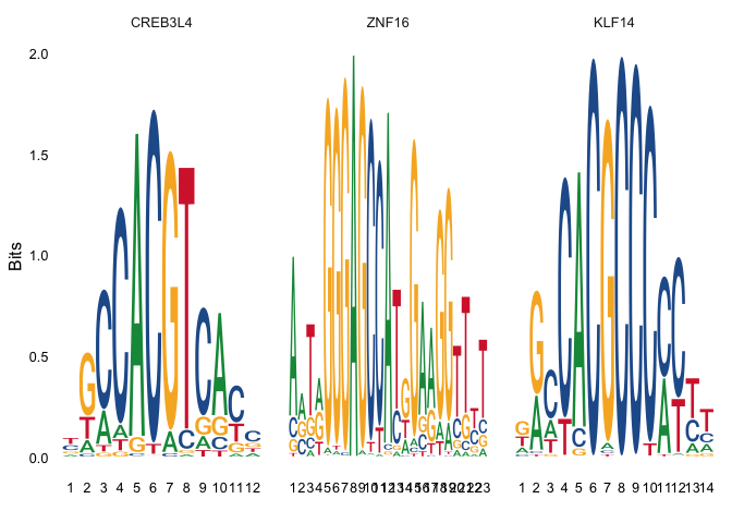
enriched.motifs <- FindMotifs(experiment.aggregate, features = top.de.peaks)
## Plot motifs
MotifPlot(experiment.aggregate, motifs = rownames(enriched.motifs)[1:3])
# read in scRNA data
scrna <- readRDS("scrna.rds")
scrna <- FindVariableFeatures(scrna)
scrna <- RunPCA(scrna)
scrna <- FindNeighbors(scrna, reduction = "pca", dims = 1:30)
scrna <- FindClusters(scrna)
## Modularity Optimizer version 1.3.0 by Ludo Waltman and Nees Jan van Eck
##
## Number of nodes: 17773
## Number of edges: 553948
##
## Running Louvain algorithm...
## Maximum modularity in 10 random starts: 0.8088
## Number of communities: 14
## Elapsed time: 2 seconds
# read in scATAC data
scatac <- readRDS("scatac.rds")
scatac <- RunTFIDF(scatac)
scatac <- FindTopFeatures(scatac, min.cutoff = 'q0')
scatac <- RunSVD(scatac)
scatac <- FindNeighbors(scatac, reduction = "lsi", dims = 2:30)
scatac <- FindClusters(scatac, algorithm = 3)
## Modularity Optimizer version 1.3.0 by Ludo Waltman and Nees Jan van Eck
##
## Number of nodes: 8737
## Number of edges: 235831
##
## Running smart local moving algorithm...
## Maximum modularity in 10 random starts: 0.6776
## Number of communities: 14
## Elapsed time: 2 seconds
At this point, we can annotate the cell types by using existing scATACSeq datasets that have been annotated with cell types and include cells that are present in the dataset of interest. There are quite a few python packages existing to accomplish this goal: Cellcano, scATAnno. Seurat, Signac, SingleR all provide functions that can be used to integrating scATAC and scRNA data and achieve cell type annotation. We are going to demonstrate one workflow.
# Signac/Seurat approach
## Generate gene activities data from scATAC data
gene.act <- GeneActivity(scatac)
scatac[['RNA']] <- CreateAssayObject(counts = gene.act)
scatac <- NormalizeData(scatac, assay = 'RNA', normalization.method = "LogNormalize")
scatac <- ScaleData(scatac, assay = 'RNA', vars.to.regress = "nCount_RNA")
saveRDS(scatac, "scatac.geneact.rds")
scatac <- readRDS("scatac.geneact.rds")
anchors <- FindTransferAnchors(reference = scrna, query = scatac, features = VariableFeatures(scrna),
        reference.assay = "RNA", query.assay = "RNA", reduction = "cca")
celltypes.atac <- TransferData(anchorset = anchors, refdata = scrna$RNA_snn_res.0.8,
        weight.reduction = scatac[["lsi"]], dims = 2:30)
sessionInfo()
## R version 4.4.0 (2024-04-24)
## Platform: aarch64-apple-darwin20
## Running under: macOS Ventura 13.5.2
##
## Matrix products: default
## BLAS:   /Library/Frameworks/R.framework/Versions/4.4-arm64/Resources/lib/libRblas.0.dylib
## LAPACK: /Library/Frameworks/R.framework/Versions/4.4-arm64/Resources/lib/libRlapack.dylib;  LAPACK version 3.12.0
##
## locale:
## [1] en_US.UTF-8/en_US.UTF-8/en_US.UTF-8/C/en_US.UTF-8/en_US.UTF-8
##
## time zone: America/Los_Angeles
## tzcode source: internal
##
## attached base packages:
## [1] stats4    parallel  stats     graphics  grDevices utils     datasets
## [8] methods   base
##
## other attached packages:
##  [1] ggseqlogo_0.2                     TFBSTools_1.43.0
##  [3] JASPAR2020_0.99.10                chromVAR_1.27.0
##  [5] ggforce_0.4.2                     BSgenome.Hsapiens.UCSC.hg38_1.4.5
##  [7] BSgenome_1.72.0                   rtracklayer_1.64.0
##  [9] BiocIO_1.14.0                     Biostrings_2.72.0
## [11] XVector_0.44.0                    kableExtra_1.4.0
## [13] HGNChelper_0.8.14                 biovizBase_1.52.0
## [15] Signac_1.13.0                     ensembldb_2.29.0
## [17] AnnotationFilter_1.29.0           GenomicFeatures_1.57.0
## [19] AnnotationDbi_1.66.0              Biobase_2.64.0
## [21] GenomicRanges_1.56.0              GenomeInfoDb_1.40.1
## [23] IRanges_2.38.0                    S4Vectors_0.42.0
## [25] AnnotationHub_3.12.0              BiocFileCache_2.12.0
## [27] dbplyr_2.5.0                      BiocGenerics_0.50.0
## [29] ROCR_1.0-11                       KernSmooth_2.23-22
## [31] fields_15.2                       viridisLite_0.4.2
## [33] spam_2.10-0                       SoupX_1.6.2
## [35] ggplot2_3.5.1                     DoubletFinder_2.0.4
## [37] Seurat_5.1.0                      SeuratObject_5.0.2
## [39] sp_2.1-4
##
## loaded via a namespace (and not attached):
##   [1] ProtGenerics_1.37.0         matrixStats_1.3.0
##   [3] spatstat.sparse_3.0-3       bitops_1.0-7
##   [5] DirichletMultinomial_1.46.0 httr_1.4.7
##   [7] RColorBrewer_1.1-3          tools_4.4.0
##   [9] sctransform_0.4.1           backports_1.5.0
##  [11] DT_0.33                     utf8_1.2.4
##  [13] R6_2.5.1                    lazyeval_0.2.2
##  [15] uwot_0.2.2                  withr_3.0.0
##  [17] gridExtra_2.3               progressr_0.14.0
##  [19] cli_3.6.2                   spatstat.explore_3.2-7
##  [21] fastDummies_1.7.3           labeling_0.4.3
##  [23] sass_0.4.9                  spatstat.data_3.0-4
##  [25] readr_2.1.5                 ggridges_0.5.6
##  [27] pbapply_1.7-2               systemfonts_1.1.0
##  [29] Rsamtools_2.20.0            foreign_0.8-86
##  [31] R.utils_2.12.3              svglite_2.1.3
##  [33] dichromat_2.0-0.1           parallelly_1.37.1
##  [35] limma_3.60.2                maps_3.4.2
##  [37] rstudioapi_0.16.0           RSQLite_2.3.7
##  [39] generics_0.1.3              gtools_3.9.5
##  [41] ica_1.0-3                   spatstat.random_3.2-3
##  [43] zip_2.3.1                   dplyr_1.1.4
##  [45] GO.db_3.19.1                Matrix_1.7-0
##  [47] fansi_1.0.6                 abind_1.4-5
##  [49] R.methodsS3_1.8.2           lifecycle_1.0.4
##  [51] yaml_2.3.8                  SummarizedExperiment_1.34.0
##  [53] SparseArray_1.4.8           Rtsne_0.17
##  [55] grid_4.4.0                  blob_1.2.4
##  [57] promises_1.3.0              pwalign_1.0.0
##  [59] crayon_1.5.2                miniUI_0.1.1.1
##  [61] lattice_0.22-6              cowplot_1.1.3
##  [63] annotate_1.82.0             KEGGREST_1.44.0
##  [65] pillar_1.9.0                knitr_1.47
##  [67] rjson_0.2.21                future.apply_1.11.2
##  [69] codetools_0.2-20            fastmatch_1.1-4
##  [71] leiden_0.4.3.1              glue_1.7.0
##  [73] data.table_1.15.4           vctrs_0.6.5
##  [75] png_0.1-8                   poweRlaw_0.80.0
##  [77] gtable_0.3.5                cachem_1.1.0
##  [79] openxlsx_4.2.5.2            xfun_0.44
##  [81] S4Arrays_1.4.1              mime_0.12
##  [83] pracma_2.4.4                survival_3.5-8
##  [85] RcppRoll_0.3.0              statmod_1.5.0
##  [87] fitdistrplus_1.1-11         nlme_3.1-164
##  [89] bit64_4.0.5                 filelock_1.0.3
##  [91] RcppAnnoy_0.0.22            bslib_0.7.0
##  [93] irlba_2.3.5.1               rpart_4.1.23
##  [95] seqLogo_1.70.0              splitstackshape_1.4.8
##  [97] colorspace_2.1-0            DBI_1.2.3
##  [99] Hmisc_5.1-3                 nnet_7.3-19
## [101] tidyselect_1.2.1            bit_4.0.5
## [103] compiler_4.4.0              curl_5.2.1
## [105] htmlTable_2.4.2             hdf5r_1.3.10
## [107] xml2_1.3.6                  DelayedArray_0.30.1
## [109] plotly_4.10.4               caTools_1.18.2
## [111] checkmate_2.3.1             scales_1.3.0
## [113] lmtest_0.9-40               rappdirs_0.3.3
## [115] stringr_1.5.1               digest_0.6.35
## [117] goftest_1.2-3               presto_1.0.0
## [119] spatstat.utils_3.0-4        motifmatchr_1.26.0
## [121] rmarkdown_2.27              htmltools_0.5.8.1
## [123] pkgconfig_2.0.3             base64enc_0.1-3
## [125] MatrixGenerics_1.16.0       highr_0.11
## [127] fastmap_1.2.0               rlang_1.1.3
## [129] htmlwidgets_1.6.4           UCSC.utils_1.0.0
## [131] shiny_1.8.1.1               farver_2.1.2
## [133] jquerylib_0.1.4             zoo_1.8-12
## [135] jsonlite_1.8.8              BiocParallel_1.38.0
## [137] R.oo_1.26.0                 VariantAnnotation_1.50.0
## [139] RCurl_1.98-1.14             magrittr_2.0.3
## [141] Formula_1.2-5               GenomeInfoDbData_1.2.12
## [143] dotCall64_1.1-1             patchwork_1.2.0
## [145] munsell_0.5.1               Rcpp_1.0.12
## [147] reticulate_1.37.0           stringi_1.8.4
## [149] zlibbioc_1.50.0             MASS_7.3-60.2
## [151] plyr_1.8.9                  listenv_0.9.1
## [153] ggrepel_0.9.5               CNEr_1.41.0
## [155] deldir_2.0-4                splines_4.4.0
## [157] tensor_1.5                  hms_1.1.3
## [159] igraph_2.0.3                spatstat.geom_3.2-9
## [161] RcppHNSW_0.6.0              reshape2_1.4.4
## [163] TFMPvalue_0.0.9             BiocVersion_3.19.1
## [165] XML_3.99-0.16.1             evaluate_0.23
## [167] BiocManager_1.30.23         tzdb_0.4.0
## [169] tweenr_2.0.3                httpuv_1.6.15
## [171] RANN_2.6.1                  tidyr_1.3.1
## [173] purrr_1.0.2                 polyclip_1.10-6
## [175] future_1.33.2               scattermore_1.2
## [177] xtable_1.8-4                restfulr_0.0.15
## [179] RSpectra_0.16-1             later_1.3.2
## [181] tibble_3.2.1                memoise_2.0.1
## [183] GenomicAlignments_1.40.0    cluster_2.1.6
## [185] globals_0.16.3