
Differential Gene Expression Analysis in R
- Differential Gene Expression (DGE) between conditions is determined from count data
- Generally speaking differential expression analysis is performed in a very similar manner to metabolomics, proteomics, or DNA microarrays, once normalization and transformations have been performed.
A lot of RNA-seq analysis has been done in R and so there are many packages available to analyze and view this data. Two of the most commonly used are:
- DESeq2, developed by Simon Anders (also created htseq) in Wolfgang Huber’s group at EMBL
- edgeR and Voom (extension to Limma [microarrays] for RNA-seq), developed out of Gordon Smyth’s group from the Walter and Eliza Hall Institute of Medical Research in Australia
http://bioconductor.org/packages/release/BiocViews.html#___RNASeq
Differential Expression Analysis with Limma-Voom
limma is an R package that was originally developed for differential expression (DE) analysis of gene expression microarray data.
voom is a function in the limma package that transforms RNA-Seq data for use with limma.
Together they allow fast, flexible, and powerful analyses of RNA-Seq data. Limma-voom is our tool of choice for DE analyses because it:
-
Allows for incredibly flexible model specification (you can include multiple categorical and continuous variables, allowing incorporation of almost any kind of metadata).
-
Based on simulation studies, maintains the false discovery rate at or below the nominal rate, unlike some other packages.
-
Empirical Bayes smoothing of gene-wise standard deviations provides increased power.
Basic Steps of Differential Gene Expression
- Read count data and annotation into R and preprocessing.
- Calculate normalization factors (sample-specific adjustments)
- Filter genes (uninteresting genes, e.g. unexpressed)
- Account for expression-dependent variability by transformation, weighting, or modeling
- Fitting a linear model
- Perform statistical comparisons of interest (using contrasts)
- Adjust for multiple testing, Benjamini-Hochberg (BH) or q-value
- Check results for confidence
- Attach annotation if available and write tables
1. Read in the counts table and create our DGEList
counts <- read.delim("rnaseq_workshop_counts.txt", row.names = 1)
head(counts)
##                      mouse_110_WT_C mouse_110_WT_NC mouse_148_WT_C
## ENSMUSG00000102693.2              0               0              0
## ENSMUSG00000064842.3              0               0              0
## ENSMUSG00000051951.6              1               0              0
## ENSMUSG00000102851.2              0               0              0
## ENSMUSG00000103377.2              0               0              0
## ENSMUSG00000104017.2              0               0              0
##                      mouse_148_WT_NC mouse_158_WT_C mouse_158_WT_NC
## ENSMUSG00000102693.2               0              0               0
## ENSMUSG00000064842.3               0              0               0
## ENSMUSG00000051951.6               2              1               0
## ENSMUSG00000102851.2               0              0               0
## ENSMUSG00000103377.2               0              0               0
## ENSMUSG00000104017.2               0              0               0
##                      mouse_183_KOMIR150_C mouse_183_KOMIR150_NC
## ENSMUSG00000102693.2                    0                     0
## ENSMUSG00000064842.3                    0                     0
## ENSMUSG00000051951.6                    1                     1
## ENSMUSG00000102851.2                    0                     0
## ENSMUSG00000103377.2                    0                     0
## ENSMUSG00000104017.2                    0                     0
##                      mouse_198_KOMIR150_C mouse_198_KOMIR150_NC
## ENSMUSG00000102693.2                    0                     0
## ENSMUSG00000064842.3                    0                     0
## ENSMUSG00000051951.6                    1                     0
## ENSMUSG00000102851.2                    0                     0
## ENSMUSG00000103377.2                    0                     0
## ENSMUSG00000104017.2                    0                     0
##                      mouse_206_KOMIR150_C mouse_206_KOMIR150_NC
## ENSMUSG00000102693.2                    0                     0
## ENSMUSG00000064842.3                    0                     0
## ENSMUSG00000051951.6                    1                     0
## ENSMUSG00000102851.2                    0                     0
## ENSMUSG00000103377.2                    0                     0
## ENSMUSG00000104017.2                    0                     0
##                      mouse_2670_KOTet3_C mouse_2670_KOTet3_NC
## ENSMUSG00000102693.2                   0                    0
## ENSMUSG00000064842.3                   0                    0
## ENSMUSG00000051951.6                   0                    1
## ENSMUSG00000102851.2                   0                    0
## ENSMUSG00000103377.2                   0                    0
## ENSMUSG00000104017.2                   0                    0
##                      mouse_7530_KOTet3_C mouse_7530_KOTet3_NC
## ENSMUSG00000102693.2                   0                    0
## ENSMUSG00000064842.3                   0                    0
## ENSMUSG00000051951.6                   0                    1
## ENSMUSG00000102851.2                   0                    0
## ENSMUSG00000103377.2                   0                    0
## ENSMUSG00000104017.2                   0                    0
##                      mouse_7531_KOTet3_C mouse_7532_WT_NC mouse_H510_WT_C
## ENSMUSG00000102693.2                   0                0               0
## ENSMUSG00000064842.3                   0                0               0
## ENSMUSG00000051951.6                   1                0               0
## ENSMUSG00000102851.2                   0                0               0
## ENSMUSG00000103377.2                   0                0               0
## ENSMUSG00000104017.2                   0                0               0
##                      mouse_H510_WT_NC mouse_H514_WT_C mouse_H514_WT_NC
## ENSMUSG00000102693.2                0               0                0
## ENSMUSG00000064842.3                0               0                0
## ENSMUSG00000051951.6                1               0                1
## ENSMUSG00000102851.2                0               0                0
## ENSMUSG00000103377.2                0               0                0
## ENSMUSG00000104017.2                0               0                0
Create Differential Gene Expression List Object (DGEList) object
A DGEList is an object in the package edgeR for storing count data, normalization factors, and other information
d0 <- DGEList(counts)
1a. Read in Annotation
anno <- read.delim("ensembl_mm_112.txt",as.is=T)
dim(anno)
## [1] 149194 13
head(anno)
##       Gene.stable.ID Gene.stable.ID.version Transcript.stable.ID
## 1 ENSMUSG00000064336   ENSMUSG00000064336.1   ENSMUST00000082387
## 2 ENSMUSG00000064337   ENSMUSG00000064337.1   ENSMUST00000082388
## 3 ENSMUSG00000064338   ENSMUSG00000064338.1   ENSMUST00000082389
## 4 ENSMUSG00000064339   ENSMUSG00000064339.1   ENSMUST00000082390
## 5 ENSMUSG00000064340   ENSMUSG00000064340.1   ENSMUST00000082391
## 6 ENSMUSG00000064341   ENSMUSG00000064341.1   ENSMUST00000082392
##   Transcript.stable.ID.version
## 1         ENSMUST00000082387.1
## 2         ENSMUST00000082388.1
## 3         ENSMUST00000082389.1
## 4         ENSMUST00000082390.1
## 5         ENSMUST00000082391.1
## 6         ENSMUST00000082392.1
##                                                                  Gene.description
## 1   mitochondrially encoded tRNA phenylalanine [Source:MGI Symbol;Acc:MGI:102487]
## 2             mitochondrially encoded 12S rRNA [Source:MGI Symbol;Acc:MGI:102493]
## 3          mitochondrially encoded tRNA valine [Source:MGI Symbol;Acc:MGI:102472]
## 4             mitochondrially encoded 16S rRNA [Source:MGI Symbol;Acc:MGI:102492]
## 5       mitochondrially encoded tRNA leucine 1 [Source:MGI Symbol;Acc:MGI:102482]
## 6 mitochondrially encoded NADH dehydrogenase 1 [Source:MGI Symbol;Acc:MGI:101787]
##   Chromosome.scaffold.name Gene.start..bp. Gene.end..bp. Strand Gene.name
## 1                       MT               1            68      1     mt-Tf
## 2                       MT              70          1024      1   mt-Rnr1
## 3                       MT            1025          1093      1     mt-Tv
## 4                       MT            1094          2675      1   mt-Rnr2
## 5                       MT            2676          2750      1    mt-Tl1
## 6                       MT            2751          3707      1    mt-Nd1
##   Transcript.count Gene...GC.content      Gene.type
## 1                1             30.88        Mt_tRNA
## 2                1             35.81        Mt_rRNA
## 3                1             39.13        Mt_tRNA
## 4                1             35.40        Mt_rRNA
## 5                1             44.00        Mt_tRNA
## 6                1             37.62 protein_coding
tail(anno)
##            Gene.stable.ID Gene.stable.ID.version Transcript.stable.ID
## 149189 ENSMUSG00000087600   ENSMUSG00000087600.3   ENSMUST00000150185
## 149190 ENSMUSG00000025314  ENSMUSG00000025314.19   ENSMUST00000129323
## 149191 ENSMUSG00000025314  ENSMUSG00000025314.19   ENSMUST00000111495
## 149192 ENSMUSG00000025314  ENSMUSG00000025314.19   ENSMUST00000168621
## 149193 ENSMUSG00000085471   ENSMUSG00000085471.2   ENSMUST00000126219
## 149194 ENSMUSG00000085471   ENSMUSG00000085471.2   ENSMUST00000126953
##        Transcript.stable.ID.version
## 149189         ENSMUST00000150185.2
## 149190         ENSMUST00000129323.2
## 149191         ENSMUST00000111495.9
## 149192         ENSMUST00000168621.5
## 149193         ENSMUST00000126219.2
## 149194         ENSMUST00000126953.2
##                                                                                               Gene.description
## 149189 prostate transmembrane protein, androgen induced 1, opposite strand [Source:MGI Symbol;Acc:MGI:3650161]
## 149190                         protein tyrosine phosphatase receptor type J [Source:MGI Symbol;Acc:MGI:104574]
## 149191                         protein tyrosine phosphatase receptor type J [Source:MGI Symbol;Acc:MGI:104574]
## 149192                         protein tyrosine phosphatase receptor type J [Source:MGI Symbol;Acc:MGI:104574]
## 149193     protein tyrosine phosphatase receptor type J, opposite strand 1 [Source:MGI Symbol;Acc:MGI:1918408]
## 149194     protein tyrosine phosphatase receptor type J, opposite strand 1 [Source:MGI Symbol;Acc:MGI:1918408]
##        Chromosome.scaffold.name Gene.start..bp. Gene.end..bp. Strand Gene.name
## 149189                        2       173118467     173120221      1  Pmepa1os
## 149190                        2        90260098      90410991     -1     Ptprj
## 149191                        2        90260098      90410991     -1     Ptprj
## 149192                        2        90260098      90410991     -1     Ptprj
## 149193                        2        90309580      90318769      1  Ptprjos1
## 149194                        2        90309580      90318769      1  Ptprjos1
##        Transcript.count Gene...GC.content      Gene.type
## 149189                2             50.48         lncRNA
## 149190                3             45.73 protein_coding
## 149191                3             45.73 protein_coding
## 149192                3             45.73 protein_coding
## 149193                2             46.65         lncRNA
## 149194                2             46.65         lncRNA
any(duplicated(anno$Gene.stable.ID))
## [1] TRUE
1b. Derive experiment metadata from the sample names
Our experiment has two factors, genotype (“WT”, “KOMIR150”, or “KOTet3”) and cell type (“C” or “NC”).
The sample names are “mouse” followed by an animal identifier, followed by the genotype, followed by the cell type.
sample_names <- colnames(counts)
metadata <- as.data.frame(strsplit2(sample_names, c("_"))[,2:4], row.names = sample_names)
colnames(metadata) <- c("mouse", "genotype", "cell_type")
Create a new variable “group” that combines genotype and cell type.
metadata$group <- interaction(metadata$genotype, metadata$cell_type)
table(metadata$group)
##
##  KOMIR150.C    KOTet3.C        WT.C KOMIR150.NC   KOTet3.NC       WT.NC
##           3           3           5           3           2           6
table(metadata$mouse)
##
##  110  148  158  183  198  206 2670 7530 7531 7532 H510 H514
##    2    2    2    2    2    2    2    2    1    1    2    2
Note: you can also enter group information manually, or read it in from an external file. If you do this, it is $VERY, VERY, VERY$ important that you make sure the metadata is in the same order as the column names of the counts table.
Quiz 1
2. Preprocessing and Normalization factors
In differential expression analysis, only sample-specific effects need to be normalized, we are NOT concerned with comparisons and quantification of absolute expression.
- Sequence depth – is a sample specific effect and needs to be adjusted for.
- RNA composition - finding a set of scaling factors for the library sizes that minimize the log-fold changes between the samples for most genes (edgeR uses a trimmed mean of M-values between each pair of sample)
- GC content – is NOT sample-specific (except when it is)
- Gene Length – is NOT sample-specific (except when it is)
In edgeR/limma, you calculate normalization factors to scale the raw library sizes (number of reads) using the function calcNormFactors, which by default uses TMM (weighted trimmed means of M values to the reference). Assumes most genes are not DE.
Proposed by Robinson and Oshlack (2010).
d0 <- calcNormFactors(d0)
d0$samples
##                       group lib.size norm.factors
## mouse_110_WT_C            1 12565440    1.0202749
## mouse_110_WT_NC           1 19787656    0.9827710
## mouse_148_WT_C            1 21828646    1.0191795
## mouse_148_WT_NC           1 15167634    0.9727032
## mouse_158_WT_C            1 29327303    0.9995372
## mouse_158_WT_NC           1 17622133    0.9647970
## mouse_183_KOMIR150_C      1  9985163    0.9993251
## mouse_183_KOMIR150_NC     1  6346844    0.9541147
## mouse_198_KOMIR150_C      1 19186734    0.9941313
## mouse_198_KOMIR150_NC     1 22797451    0.9830820
## mouse_206_KOMIR150_C      1  4305196    0.9607709
## mouse_206_KOMIR150_NC     1  2723038    0.9130415
## mouse_2670_KOTet3_C       1 27974927    1.0271513
## mouse_2670_KOTet3_NC      1 24984193    0.9920584
## mouse_7530_KOTet3_C       1 17057677    1.0301202
## mouse_7530_KOTet3_NC      1 33965062    0.9940217
## mouse_7531_KOTet3_C       1 23527065    1.0720990
## mouse_7532_WT_NC          1 16036142    1.0174165
## mouse_H510_WT_C           1 14306965    1.0706374
## mouse_H510_WT_NC          1 18363234    1.0321657
## mouse_H514_WT_C           1  8324060    1.0071358
## mouse_H514_WT_NC          1 16538783    1.0074983
Note: calcNormFactors doesn’t normalize the data, it just calculates normalization factors for use downstream.
3. Filtering genes
We filter genes based on non-experimental factors to reduce the number of genes/tests being conducted and therefor do not have to be accounted for in our transformation or multiple testing correction. Commonly we try to remove genes that are either a) unexpressed, or b) unchanging (low-variability).
Common filters include:
- to remove genes with a max value (X) of less then Y.
- to remove genes that are less than X normalized read counts (cpm) across a certain number of samples. Ex: rowSums(cpms <=1) < 3 , require at least 1 cpm in at least 3 samples to keep.
- A less used filter is for genes with minimum variance across all samples, so if a gene isn’t changing (constant expression) its inherently not interesting therefor no need to test.
We will use the built in function filterByExpr() to filter low-expressed genes. filterByExpr uses the experimental design to determine how many samples a gene needs to be expressed in to stay. Importantly, once this number of samples has been determined, the group information is not used in filtering.
Using filterByExpr requires specifying the model we will use to analysis our data.
- The model you use will change for every experiment, and this step should be given the most time and attention.*
We use a model that includes group and (in order to account for the paired design) mouse.
group <- metadata$group
mouse <- metadata$mouse
mm <- model.matrix(~0 + group + mouse)
head(mm)
##   groupKOMIR150.C groupKOTet3.C groupWT.C groupKOMIR150.NC groupKOTet3.NC
## 1               0             0         1                0              0
## 2               0             0         0                0              0
## 3               0             0         1                0              0
## 4               0             0         0                0              0
## 5               0             0         1                0              0
## 6               0             0         0                0              0
##   groupWT.NC mouse148 mouse158 mouse183 mouse198 mouse206 mouse2670 mouse7530
## 1          0        0        0        0        0        0         0         0
## 2          1        0        0        0        0        0         0         0
## 3          0        1        0        0        0        0         0         0
## 4          1        1        0        0        0        0         0         0
## 5          0        0        1        0        0        0         0         0
## 6          1        0        1        0        0        0         0         0
##   mouse7531 mouse7532 mouseH510 mouseH514
## 1         0         0         0         0
## 2         0         0         0         0
## 3         0         0         0         0
## 4         0         0         0         0
## 5         0         0         0         0
## 6         0         0         0         0
keep <- filterByExpr(d0, mm)
sum(keep) # number of genes retained
## [1] 16093
d <- d0[keep,]
“Low-expressed” depends on the dataset and can be subjective.
Visualizing your data with a Multidimensional scaling (MDS) plot.
plotMDS(d, col = as.numeric(metadata$group), cex=1)
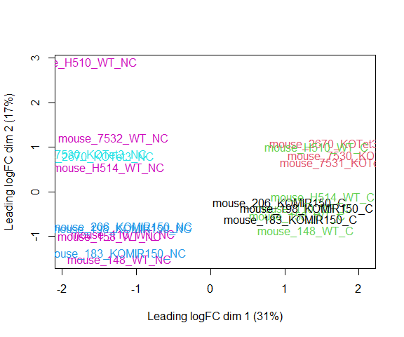
The MDS plot tells you A LOT about what to expect from your experiment.
3a. Extracting “normalized” expression table
RPKM vs. FPKM vs. CPM and Model Based
- RPKM - Reads per kilobase per million mapped reads
- FPKM - Fragments per kilobase per million mapped reads
- logCPM – log Counts per million [ good for producing MDS plots, estimate of normalized values in model based ]
- Model based - original read counts are not themselves transformed, but rather correction factors are used in the DE model itself.
We use the cpm function with log=TRUE to obtain log-transformed normalized expression data. On the log scale, the data has less mean-dependent variability and is more suitable for plotting.
logcpm <- cpm(d, prior.count=2, log=TRUE)
write.table(logcpm,"rnaseq_workshop_normalized_counts.txt",sep="\t",quote=F)
Quiz 2
4. Voom transformation and calculation of variance weights
4a. Voom
y <- voom(d, mm, plot = T)
## Coefficients not estimable: mouse206 mouse7531
## Warning: Partial NA coefficients for 16093 probe(s)
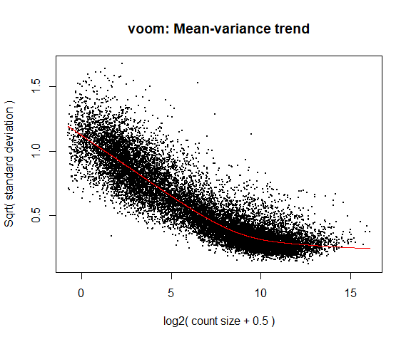
What is voom doing?
- Counts are transformed to log2 counts per million reads (CPM), where “per million reads” is defined based on the normalization factors we calculated earlier.
- A linear model is fitted to the log2 CPM for each gene, and the residuals are calculated.
- A smoothed curve is fitted to the sqrt(residual standard deviation) by average expression. (see red line in plot above)
- The smoothed curve is used to obtain weights for each gene and sample that are passed into limma along with the log2 CPMs.
More details at “voom: precision weights unlock linear model analysis tools for RNA-seq read counts”
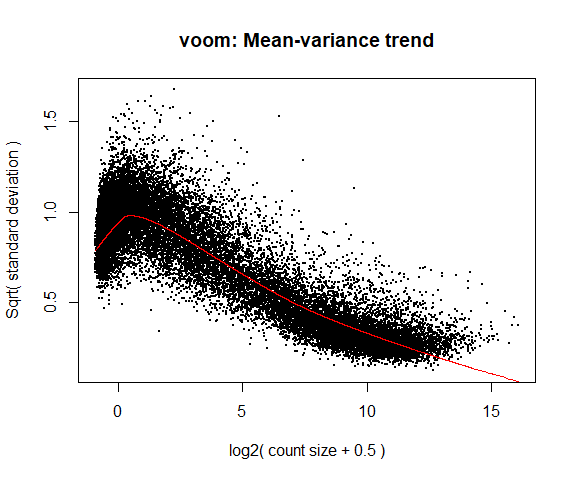
If your voom plot looks like the below (performed on the raw data), you might want to filter more:
tmp <- voom(d0, mm, plot = T)
## Coefficients not estimable: mouse206 mouse7531
## Warning: Partial NA coefficients for 57132 probe(s)
5. Fitting linear models in limma
lmFit fits a linear model using weighted least squares for each gene:
fit <- lmFit(y, mm)
## Coefficients not estimable: mouse206 mouse7531
## Warning: Partial NA coefficients for 16093 probe(s)
head(coef(fit))
##                       groupKOMIR150.C groupKOTet3.C  groupWT.C groupKOMIR150.NC
## ENSMUSG00000098104.2        0.6167106   -0.04197779  0.6168613        0.2225588
## ENSMUSG00000033845.14       5.1178809    4.94971758  5.0045344        5.1110565
## ENSMUSG00000102275.2       -1.6387447   -0.70249132 -1.2393623       -1.1558881
## ENSMUSG00000025903.15       5.2448220    5.53622159  5.5163295        5.3252042
## ENSMUSG00000033813.16       5.8116828    5.63275495  5.8367118        5.8830626
## ENSMUSG00000033793.13       5.2373320    5.35803030  5.3157875        5.0975290
##                       groupKOTet3.NC  groupWT.NC    mouse148    mouse158
## ENSMUSG00000098104.2      -0.3456633  0.06098638 -0.99761877 -0.40390363
## ENSMUSG00000033845.14      4.6695809  4.88877173 -0.15050881 -0.03346697
## ENSMUSG00000102275.2      -1.5403946 -1.02042710 -0.36288740  0.26697669
## ENSMUSG00000025903.15      5.5695393  5.42227852  0.13356006  0.12996746
## ENSMUSG00000033813.16      5.7119106  5.83434627 -0.03924021 -0.05980918
## ENSMUSG00000033793.13      5.0045858  5.11188806  0.11459381  0.03028331
##                          mouse183    mouse198 mouse206  mouse2670   mouse7530
## ENSMUSG00000098104.2   0.06485518 -0.89229010       NA  0.1240240 -0.17489546
## ENSMUSG00000033845.14 -0.39137385 -0.08530003       NA  0.2659305  0.17631873
## ENSMUSG00000102275.2   1.12152352  0.09294231       NA -0.2464155 -0.23811543
## ENSMUSG00000025903.15  0.23511232  0.30190559       NA  0.1302013  0.09593625
## ENSMUSG00000033813.16 -0.11996066  0.03357792       NA  0.2692394  0.21713345
## ENSMUSG00000033793.13 -0.01321460  0.15273643       NA  0.2817415  0.41272767
##                       mouse7531   mouse7532   mouseH510    mouseH514
## ENSMUSG00000098104.2         NA -0.84122451 -0.49562157 -0.233961069
## ENSMUSG00000033845.14        NA -0.01456226 -0.02259506  0.005335215
## ENSMUSG00000102275.2         NA  1.03665557 -0.14330584 -0.227521278
## ENSMUSG00000025903.15        NA  0.17800137  0.12243961  0.128254857
## ENSMUSG00000033813.16        NA -0.03199671 -0.01798841 -0.040208157
## ENSMUSG00000033793.13        NA  0.04606053  0.09850559  0.088652873
Comparisons between groups (log fold-changes) are obtained as contrasts of these fitted linear models:
6. Specify which groups to compare using contrasts:
Comparison between cell types for genotype WT.
contr <- makeContrasts(groupWT.C - groupWT.NC, levels = colnames(coef(fit)))
contr
##                   Contrasts
## Levels             groupWT.C - groupWT.NC
##   groupKOMIR150.C                       0
##   groupKOTet3.C                         0
##   groupWT.C                             1
##   groupKOMIR150.NC                      0
##   groupKOTet3.NC                        0
##   groupWT.NC                           -1
##   mouse148                              0
##   mouse158                              0
##   mouse183                              0
##   mouse198                              0
##   mouse206                              0
##   mouse2670                             0
##   mouse7530                             0
##   mouse7531                             0
##   mouse7532                             0
##   mouseH510                             0
##   mouseH514                             0
6a. Estimate contrast for each gene
tmp <- contrasts.fit(fit, contr)
The variance characteristics of low expressed genes are different from high expressed genes, if treated the same, the effect is to over represent low expressed genes in the DE list. This is corrected for by the log transformation and voom. However, some genes will have increased or decreased variance that is not a result of low expression, but due to other random factors. We are going to run empirical Bayes to adjust the variance of these genes.
Empirical Bayes smoothing of standard errors (shifts standard errors that are much larger or smaller than those from other genes towards the average standard error) (see “Linear Models and Empirical Bayes Methods for Assessing Differential Expression in Microarray Experiments”
6b. Apply EBayes
tmp <- eBayes(tmp)
7. Multiple Testing Adjustment
The TopTable. Adjust for multiple testing using method of Benjamini & Hochberg (BH), or its ‘alias’ fdr. “Controlling the false discovery rate: a practical and powerful approach to multiple testing.
here n=Inf says to produce the topTable for all genes.
top.table <- topTable(tmp, adjust.method = "BH", sort.by = "P", n = Inf)
Multiple Testing Correction
Simply a must! Best choices are:
The FDR (or qvalue) is a statement about the list and is no longer about the gene (pvalue). So a FDR of 0.05, says you expect 5% false positives among the list of genes with an FDR of 0.05 or less.
The statement “Statistically significantly different” means FDR of 0.05 or less.
7a. How many DE genes are there (false discovery rate corrected)?
length(which(top.table$adj.P.Val < 0.05))
## [1] 8332
8. Check your results for confidence.
You’ve conducted an experiment, you’ve seen a phenotype. Now check which genes are most differentially expressed (show the top 50)? Look up these top genes, their description and ensure they relate to your experiment/phenotype.
head(top.table, 50)
##                           logFC   AveExpr         t      P.Value    adj.P.Val
## ENSMUSG00000033530.9  -2.042255  5.737889 -47.93788 1.705584e-15 1.423607e-11
## ENSMUSG00000051177.17  3.062891  5.181219  46.30958 2.616034e-15 1.423607e-11
## ENSMUSG00000020608.8  -2.306549  7.921139 -45.51885 3.237429e-15 1.423607e-11
## ENSMUSG00000027508.16 -1.796391  8.219229 -44.63348 4.128023e-15 1.423607e-11
## ENSMUSG00000027215.14 -2.476432  6.888318 -44.38509 4.423061e-15 1.423607e-11
## ENSMUSG00000049103.15  1.972002  9.750359  41.37645 1.053529e-14 2.825740e-11
## ENSMUSG00000028497.13  1.601384  7.098445  40.66526 1.305254e-14 3.000780e-11
## ENSMUSG00000023827.9  -1.918308  6.529807 -38.70750 2.400904e-14 4.434804e-11
## ENSMUSG00000030342.9  -3.320326  6.016661 -38.45189 2.605567e-14 4.434804e-11
## ENSMUSG00000025701.13 -2.545703  5.561910 -38.27776 2.755735e-14 4.434804e-11
## ENSMUSG00000020212.15 -2.113301  6.919176 -36.96762 4.235508e-14 5.464985e-11
## ENSMUSG00000041268.18  2.453719  5.112961  36.61842 4.761667e-14 5.464985e-11
## ENSMUSG00000028885.9  -2.254506  7.122811 -36.61316 4.770113e-14 5.464985e-11
## ENSMUSG00000054676.18  2.196162  6.216301  36.45324 5.034767e-14 5.464985e-11
## ENSMUSG00000021614.17  5.584311  5.834326  36.41880 5.093816e-14 5.464985e-11
## ENSMUSG00000009739.19 -3.477309  3.378294 -36.00731 5.860167e-14 5.894230e-11
## ENSMUSG00000038147.15  1.570467  7.200531  35.65803 6.608655e-14 5.934117e-11
## ENSMUSG00000038807.20 -1.509480  9.050186 -35.64552 6.637302e-14 5.934117e-11
## ENSMUSG00000024193.9  -1.510462  6.209510 -35.23610 7.653283e-14 6.482330e-11
## ENSMUSG00000042700.17 -1.804190  6.227048 -34.40859 1.025779e-13 8.253930e-11
## ENSMUSG00000024548.12 -4.649711  3.887105 -33.62469 1.362558e-13 1.017029e-10
## ENSMUSG00000111792.2  -1.869714  5.896711 -33.56964 1.390333e-13 1.017029e-10
## ENSMUSG00000020437.13 -1.106134 10.232543 -33.04963 1.685041e-13 1.141394e-10
## ENSMUSG00000068329.13 -1.488880  6.842551 -33.02245 1.702197e-13 1.141394e-10
## ENSMUSG00000052212.7   4.321302  6.402789  32.66721 1.944619e-13 1.230795e-10
## ENSMUSG00000023809.12 -3.182496  5.042599 -32.60807 1.988484e-13 1.230795e-10
## ENSMUSG00000102418.2  -2.540020  5.474824 -32.46809 2.096613e-13 1.249659e-10
## ENSMUSG00000030203.18 -4.030843  7.065843 -32.23202 2.293609e-13 1.318252e-10
## ENSMUSG00000037185.10 -1.361033  9.394521 -31.51989 3.019181e-13 1.667321e-10
## ENSMUSG00000022637.12 -1.341454  7.392963 -31.44554 3.108161e-13 1.667321e-10
## ENSMUSG00000016498.11 -4.354534  2.369451 -31.25632 3.347637e-13 1.737856e-10
## ENSMUSG00000021322.9   4.280777  4.359665  31.16153 3.475041e-13 1.747620e-10
## ENSMUSG00000041754.6  -1.923801  5.480885 -30.41281 4.685926e-13 2.225361e-10
## ENSMUSG00000008496.20 -1.368938  9.476946 -30.35402 4.798685e-13 2.225361e-10
## ENSMUSG00000021242.10  1.594750  8.840715  30.33293 4.839847e-13 2.225361e-10
## ENSMUSG00000033705.18  1.641969  7.294086  30.15033 5.212571e-13 2.330164e-10
## ENSMUSG00000102037.2  -3.072884  3.415088 -29.80288 6.010233e-13 2.614126e-10
## ENSMUSG00000023942.16 -1.813730  6.002309 -29.70402 6.260573e-13 2.651353e-10
## ENSMUSG00000060044.9  -3.214537  5.148400 -29.49237 6.835211e-13 2.813067e-10
## ENSMUSG00000026473.17  1.252626  7.651740  29.43794 6.992026e-13 2.813067e-10
## ENSMUSG00000022584.15  4.320005  6.717103  29.05374 8.215720e-13 3.188173e-10
## ENSMUSG00000044783.17 -1.612354  7.098014 -29.02373 8.320590e-13 3.188173e-10
## ENSMUSG00000026923.16  1.940986  6.799936  28.93586 8.636049e-13 3.216200e-10
## ENSMUSG00000093739.2  -4.460372  1.946052 -28.84046 8.993258e-13 3.216200e-10
## ENSMUSG00000034731.12 -1.756397  6.751196 -28.84045 8.993289e-13 3.216200e-10
## ENSMUSG00000021728.9   1.505277  8.263338  28.73396 9.410968e-13 3.249327e-10
## ENSMUSG00000048498.9  -5.247504  6.600616 -28.67042 9.670084e-13 3.249327e-10
## ENSMUSG00000037820.16 -3.914156  7.259650 -28.63251 9.828385e-13 3.249327e-10
## ENSMUSG00000024164.16  1.612449  9.811738  28.61709 9.893558e-13 3.249327e-10
## ENSMUSG00000053559.14 -3.118301  3.950991 -27.96433 1.312994e-12 4.226004e-10
##                              B
## ENSMUSG00000033530.9  25.86590
## ENSMUSG00000051177.17 25.20231
## ENSMUSG00000020608.8  25.47647
## ENSMUSG00000027508.16 25.24160
## ENSMUSG00000027215.14 25.11455
## ENSMUSG00000049103.15 24.29222
## ENSMUSG00000028497.13 24.09023
## ENSMUSG00000023827.9  23.47058
## ENSMUSG00000030342.9  23.31819
## ENSMUSG00000025701.13 23.24308
## ENSMUSG00000020212.15 22.91909
## ENSMUSG00000041268.18 22.63661
## ENSMUSG00000028885.9  22.80025
## ENSMUSG00000054676.18 22.73492
## ENSMUSG00000021614.17 22.46466
## ENSMUSG00000009739.19 21.55369
## ENSMUSG00000038147.15 22.46896
## ENSMUSG00000038807.20 22.42804
## ENSMUSG00000024193.9  22.32539
## ENSMUSG00000042700.17 22.03240
## ENSMUSG00000024548.12 20.90200
## ENSMUSG00000111792.2  21.70692
## ENSMUSG00000020437.13 21.42218
## ENSMUSG00000068329.13 21.52287
## ENSMUSG00000052212.7  21.39620
## ENSMUSG00000023809.12 21.26892
## ENSMUSG00000102418.2  21.29873
## ENSMUSG00000030203.18 21.23066
## ENSMUSG00000037185.10 20.84873
## ENSMUSG00000022637.12 20.89099
## ENSMUSG00000016498.11 19.05626
## ENSMUSG00000021322.9  20.38736
## ENSMUSG00000041754.6  20.51065
## ENSMUSG00000008496.20 20.35997
## ENSMUSG00000021242.10 20.37523
## ENSMUSG00000033705.18 20.35440
## ENSMUSG00000102037.2  19.73665
## ENSMUSG00000023942.16 20.22596
## ENSMUSG00000060044.9  20.12753
## ENSMUSG00000026473.17 20.03475
## ENSMUSG00000022584.15 19.94714
## ENSMUSG00000044783.17 19.89337
## ENSMUSG00000026923.16 19.85525
## ENSMUSG00000093739.2  18.09072
## ENSMUSG00000034731.12 19.83104
## ENSMUSG00000021728.9  19.71295
## ENSMUSG00000048498.9  19.79678
## ENSMUSG00000037820.16 19.75919
## ENSMUSG00000024164.16 19.59325
## ENSMUSG00000053559.14 19.28623
Columns are
- logFC: log2 fold change of WT.C/WT.NC
- AveExpr: Average expression across all samples, in log2 CPM
- t: logFC divided by its standard error
- P.Value: Raw p-value (based on t) from test that logFC differs from 0
- adj.P.Val: Benjamini-Hochberg false discovery rate adjusted p-value
- B: log-odds that gene is DE (arguably less useful than the other columns)
ENSMUSG00000030203.18 has higher expression at WT NC than at WT C (logFC is negative). ENSMUSG00000026193.16 has higher expression at WT C than at WT NC (logFC is positive).
9. Write top.table to a file, adding in cpms and annotation
top.table$Gene <- rownames(top.table)
top.table <- top.table[,c("Gene", names(top.table)[1:6])]
top.table <- data.frame(top.table,anno[match(top.table$Gene,anno$Gene.stable.ID.version),],logcpm[match(top.table$Gene,rownames(logcpm)),])

head(top.table)
##                                        Gene     logFC  AveExpr         t
## ENSMUSG00000033530.9   ENSMUSG00000033530.9 -2.042255 5.737889 -47.93788
## ENSMUSG00000051177.17 ENSMUSG00000051177.17  3.062891 5.181219  46.30958
## ENSMUSG00000020608.8   ENSMUSG00000020608.8 -2.306549 7.921139 -45.51885
## ENSMUSG00000027508.16 ENSMUSG00000027508.16 -1.796391 8.219229 -44.63348
## ENSMUSG00000027215.14 ENSMUSG00000027215.14 -2.476432 6.888318 -44.38509
## ENSMUSG00000049103.15 ENSMUSG00000049103.15  1.972002 9.750359  41.37645
##                            P.Value    adj.P.Val        B     Gene.stable.ID
## ENSMUSG00000033530.9  1.705584e-15 1.423607e-11 25.86590 ENSMUSG00000033530
## ENSMUSG00000051177.17 2.616034e-15 1.423607e-11 25.20231 ENSMUSG00000051177
## ENSMUSG00000020608.8  3.237429e-15 1.423607e-11 25.47647 ENSMUSG00000020608
## ENSMUSG00000027508.16 4.128023e-15 1.423607e-11 25.24160 ENSMUSG00000027508
## ENSMUSG00000027215.14 4.423061e-15 1.423607e-11 25.11455 ENSMUSG00000027215
## ENSMUSG00000049103.15 1.053529e-14 2.825740e-11 24.29222 ENSMUSG00000049103
##                       Gene.stable.ID.version Transcript.stable.ID
## ENSMUSG00000033530.9    ENSMUSG00000033530.9   ENSMUST00000062957
## ENSMUSG00000051177.17  ENSMUSG00000051177.17   ENSMUST00000131552
## ENSMUSG00000020608.8    ENSMUSG00000020608.8   ENSMUST00000020931
## ENSMUSG00000027508.16  ENSMUSG00000027508.16   ENSMUST00000161949
## ENSMUSG00000027215.14  ENSMUSG00000027215.14   ENSMUST00000099696
## ENSMUSG00000049103.15  ENSMUSG00000049103.15   ENSMUST00000171719
##                       Transcript.stable.ID.version
## ENSMUSG00000033530.9          ENSMUST00000062957.8
## ENSMUSG00000051177.17         ENSMUST00000131552.5
## ENSMUSG00000020608.8          ENSMUST00000020931.6
## ENSMUSG00000027508.16         ENSMUST00000161949.8
## ENSMUSG00000027215.14         ENSMUST00000099696.8
## ENSMUSG00000049103.15         ENSMUST00000171719.8
##                                                                                                          Gene.description
## ENSMUSG00000033530.9                               tetratricopeptide repeat domain 7B [Source:MGI Symbol;Acc:MGI:2144724]
## ENSMUSG00000051177.17                                           phospholipase C, beta 1 [Source:MGI Symbol;Acc:MGI:97613]
## ENSMUSG00000020608.8                          structural maintenance of chromosomes 6 [Source:MGI Symbol;Acc:MGI:1914491]
## ENSMUSG00000027508.16 phosphoprotein associated with glycosphingolipid microdomains 1 [Source:MGI Symbol;Acc:MGI:2443160]
## ENSMUSG00000027215.14                                                     CD82 antigen [Source:MGI Symbol;Acc:MGI:104651]
## ENSMUSG00000049103.15                                   C-C motif chemokine receptor 2 [Source:MGI Symbol;Acc:MGI:106185]
##                       Chromosome.scaffold.name Gene.start..bp. Gene.end..bp.
## ENSMUSG00000033530.9                        12       100267029     100487085
## ENSMUSG00000051177.17                        2       134627987     135317178
## ENSMUSG00000020608.8                        12        11315887      11369786
## ENSMUSG00000027508.16                        3         9752539       9898739
## ENSMUSG00000027215.14                        2        93249456      93293485
## ENSMUSG00000049103.15                        9       123901987     123913594
##                       Strand Gene.name Transcript.count Gene...GC.content
## ENSMUSG00000033530.9      -1     Ttc7b               10             46.68
## ENSMUSG00000051177.17      1     Plcb1                8             40.03
## ENSMUSG00000020608.8       1      Smc6               12             38.40
## ENSMUSG00000027508.16     -1      Pag1                5             44.66
## ENSMUSG00000027215.14     -1      Cd82               11             53.35
## ENSMUSG00000049103.15      1      Ccr2                4             38.86
##                            Gene.type mouse_110_WT_C mouse_110_WT_NC
## ENSMUSG00000033530.9  protein_coding       4.852840        6.874766
## ENSMUSG00000051177.17 protein_coding       6.599801        3.507881
## ENSMUSG00000020608.8  protein_coding       6.859261        9.094970
## ENSMUSG00000027508.16 protein_coding       7.322090        9.087762
## ENSMUSG00000027215.14 protein_coding       5.566306        7.973932
## ENSMUSG00000049103.15 protein_coding      10.778793        8.754068
##                       mouse_148_WT_C mouse_148_WT_NC mouse_158_WT_C
## ENSMUSG00000033530.9        4.869934        6.874964       4.853303
## ENSMUSG00000051177.17       6.650203        3.427019       6.527026
## ENSMUSG00000020608.8        7.085031        9.417168       7.022959
## ENSMUSG00000027508.16       7.257261        9.105987       7.549176
## ENSMUSG00000027215.14       5.739415        8.164020       5.807159
## ENSMUSG00000049103.15      10.896474        8.932324      10.758847
##                       mouse_158_WT_NC mouse_183_KOMIR150_C
## ENSMUSG00000033530.9         6.888907             4.816328
## ENSMUSG00000051177.17        3.570175             6.731226
## ENSMUSG00000020608.8         9.126088             6.989685
## ENSMUSG00000027508.16        9.306438             7.372180
## ENSMUSG00000027215.14        8.224685             5.736847
## ENSMUSG00000049103.15        8.700684            10.908664
##                       mouse_183_KOMIR150_NC mouse_198_KOMIR150_C
## ENSMUSG00000033530.9               6.841954             4.834387
## ENSMUSG00000051177.17              3.439356             6.952356
## ENSMUSG00000020608.8               9.366316             6.662466
## ENSMUSG00000027508.16              8.903409             7.252850
## ENSMUSG00000027215.14              8.045304             5.697997
## ENSMUSG00000049103.15              8.800304            10.503072
##                       mouse_198_KOMIR150_NC mouse_206_KOMIR150_C
## ENSMUSG00000033530.9               6.867270             4.887967
## ENSMUSG00000051177.17              4.043474             6.589992
## ENSMUSG00000020608.8               8.942380             6.674369
## ENSMUSG00000027508.16              8.865660             7.195954
## ENSMUSG00000027215.14              8.133705             5.655368
## ENSMUSG00000049103.15              8.480061            10.744949
##                       mouse_206_KOMIR150_NC mouse_2670_KOTet3_C
## ENSMUSG00000033530.9               6.911401            4.737017
## ENSMUSG00000051177.17              3.402133            7.102662
## ENSMUSG00000020608.8               8.961321            6.757653
## ENSMUSG00000027508.16              8.954319            7.861629
## ENSMUSG00000027215.14              8.026512            5.773931
## ENSMUSG00000049103.15              8.827223           11.015849
##                       mouse_2670_KOTet3_NC mouse_7530_KOTet3_C
## ENSMUSG00000033530.9              6.966067            4.592778
## ENSMUSG00000051177.17             3.237872            7.026603
## ENSMUSG00000020608.8              9.384133            6.513201
## ENSMUSG00000027508.16             9.453685            7.609674
## ENSMUSG00000027215.14             8.899676            5.839261
## ENSMUSG00000049103.15             7.517617           10.896884
##                       mouse_7530_KOTet3_NC mouse_7531_KOTet3_C mouse_7532_WT_NC
## ENSMUSG00000033530.9              6.895598            4.359784         6.447428
## ENSMUSG00000051177.17             3.275174            7.136866         3.671320
## ENSMUSG00000020608.8              9.236110            6.259101         8.851200
## ENSMUSG00000027508.16             9.398522            7.364944         8.954090
## ENSMUSG00000027215.14             8.643648            5.306034         7.818054
## ENSMUSG00000049103.15             7.339694           10.927684         9.454121
##                       mouse_H510_WT_C mouse_H510_WT_NC mouse_H514_WT_C
## ENSMUSG00000033530.9         4.275981         6.384172        4.604575
## ENSMUSG00000051177.17        6.991956         4.096156        6.651769
## ENSMUSG00000020608.8         6.453857         8.930996        6.625866
## ENSMUSG00000027508.16        6.926876         8.765084        7.276702
## ENSMUSG00000027215.14        5.175971         7.839775        5.498344
## ENSMUSG00000049103.15       11.069068         9.334558       10.982724
##                       mouse_H514_WT_NC
## ENSMUSG00000033530.9          6.653024
## ENSMUSG00000051177.17         3.456369
## ENSMUSG00000020608.8          9.064253
## ENSMUSG00000027508.16         9.047824
## ENSMUSG00000027215.14         8.005140
## ENSMUSG00000049103.15         8.888147
write.table(top.table, file = "WT.C_v_WT.NC.txt", row.names = F, sep = "\t", quote = F)
Quiz 3
Linear models and contrasts
Let’s say we want to compare genotypes for cell type C. The only thing we have to change is the call to makeContrasts:
contr <- makeContrasts(groupWT.C - groupKOMIR150.C, levels = colnames(coef(fit)))
tmp <- contrasts.fit(fit, contr)
tmp <- eBayes(tmp)
top.table <- topTable(tmp, sort.by = "P", n = Inf)
head(top.table, 20)
##                            logFC  AveExpr          t      P.Value    adj.P.Val
## ENSMUSG00000030703.9  -2.8399478 4.885325 -19.629692 9.780415e-11 1.573962e-06
## ENSMUSG00000008348.10 -1.2275084 6.095635 -11.660132 4.620046e-08 2.686875e-04
## ENSMUSG00000066687.6  -1.9090975 5.092762 -11.578256 5.008776e-08 2.686875e-04
## ENSMUSG00000044229.10 -3.1055383 6.977232 -10.844181 1.056663e-07 3.648394e-04
## ENSMUSG00000030748.10  1.7577412 7.171213  10.632602 1.320532e-07 3.648394e-04
## ENSMUSG00000032012.10 -4.7571972 5.240101 -10.604739 1.360241e-07 3.648394e-04
## ENSMUSG00000028619.16  2.6603504 4.831631   9.753528 3.471282e-07 7.980476e-04
## ENSMUSG00000028037.14  4.6862158 2.935621   9.546088 4.404515e-07 8.860233e-04
## ENSMUSG00000094344.2   3.9034739 2.055096   8.833246 1.030372e-06 1.842419e-03
## ENSMUSG00000070372.12 -0.7611305 7.365446  -8.371010 1.838377e-06 2.650231e-03
## ENSMUSG00000035212.15 -0.6796192 7.135616  -8.347081 1.895502e-06 2.650231e-03
## ENSMUSG00000096768.10 -1.7260387 3.489560  -8.289017 2.042143e-06 2.650231e-03
## ENSMUSG00000121395.1  -5.0668383 1.490256  -8.252379 2.140868e-06 2.650231e-03
## ENSMUSG00000055994.16 -0.9977129 5.992532  -8.077143 2.688843e-06 3.090825e-03
## ENSMUSG00000028028.12  0.8525587 7.393449   7.923951 3.291078e-06 3.416647e-03
## ENSMUSG00000042105.19 -0.7275783 7.559774  -7.900146 3.396903e-06 3.416647e-03
## ENSMUSG00000045382.7  -0.9306364 8.228762  -7.657291 4.709432e-06 4.458170e-03
## ENSMUSG00000031431.14 -0.6174177 8.795253  -7.277358 7.964437e-06 7.120649e-03
## ENSMUSG00000100801.2   2.3438694 5.616654   6.828813 1.516031e-05 1.284078e-02
## ENSMUSG00000034342.10 -0.5313346 9.422628  -6.764919 1.665147e-05 1.339861e-02
##                               B
## ENSMUSG00000030703.9  14.827100
## ENSMUSG00000008348.10  9.067953
## ENSMUSG00000066687.6   8.936403
## ENSMUSG00000044229.10  8.231832
## ENSMUSG00000030748.10  8.054861
## ENSMUSG00000032012.10  7.802583
## ENSMUSG00000028619.16  6.477208
## ENSMUSG00000028037.14  5.858731
## ENSMUSG00000094344.2   3.557214
## ENSMUSG00000070372.12  5.245961
## ENSMUSG00000035212.15  5.200801
## ENSMUSG00000096768.10  5.314994
## ENSMUSG00000121395.1   2.761181
## ENSMUSG00000055994.16  4.991082
## ENSMUSG00000028028.12  4.628736
## ENSMUSG00000042105.19  4.537117
## ENSMUSG00000045382.7   4.130444
## ENSMUSG00000031431.14  3.527090
## ENSMUSG00000100801.2   3.418604
## ENSMUSG00000034342.10  2.733756
length(which(top.table$adj.P.Val < 0.05)) # number of DE genes
## [1] 57
top.table$Gene <- rownames(top.table)
top.table <- top.table[,c("Gene", names(top.table)[1:6])]
top.table <- data.frame(top.table,anno[match(top.table$Gene,anno$Gene.stable.ID),],logcpm[match(top.table$Gene,rownames(logcpm)),])

write.table(top.table, file = "WT.C_v_KOMIR150.C.txt", row.names = F, sep = "\t", quote = F)
What if we refit our model as a two-factor model (rather than using the group variable)?
Create new model matrix:
genotype <- factor(metadata$genotype, levels = c("WT", "KOMIR150", "KOTet3"))
cell_type <- factor(metadata$cell_type, levels = c("C", "NC"))
mouse <- factor(metadata$mouse, levels = c("110", "148", "158", "183", "198", "206", "2670", "7530", "7531", "7532", "H510", "H514"))
mm <- model.matrix(~genotype*cell_type + mouse)
We are specifying that model includes effects for genotype, cell type, and the genotype-cell type interaction (which allows the differences between genotypes to differ across cell types).
colnames(mm)
##  [1] "(Intercept)"                  "genotypeKOMIR150"
##  [3] "genotypeKOTet3"               "cell_typeNC"
##  [5] "mouse148"                     "mouse158"
##  [7] "mouse183"                     "mouse198"
##  [9] "mouse206"                     "mouse2670"
## [11] "mouse7530"                    "mouse7531"
## [13] "mouse7532"                    "mouseH510"
## [15] "mouseH514"                    "genotypeKOMIR150:cell_typeNC"
## [17] "genotypeKOTet3:cell_typeNC"
y <- voom(d, mm, plot = F)
## Coefficients not estimable: mouse206 mouse7531
## Warning: Partial NA coefficients for 16093 probe(s)
fit <- lmFit(y, mm)
## Coefficients not estimable: mouse206 mouse7531
## Warning: Partial NA coefficients for 16093 probe(s)
head(coef(fit))
##                       (Intercept) genotypeKOMIR150 genotypeKOTet3  cell_typeNC
## ENSMUSG00000098104.2    0.6168613    -0.0001506715    -0.65883909 -0.555874923
## ENSMUSG00000033845.14   5.0045344     0.1133464642    -0.05481686 -0.115762711
## ENSMUSG00000102275.2   -1.2393623    -0.3993824054     0.53687100  0.218935214
## ENSMUSG00000025903.15   5.5163295    -0.2715074956     0.01989209 -0.094050987
## ENSMUSG00000033813.16   5.8367118    -0.0250290079    -0.20395689 -0.002365573
## ENSMUSG00000033793.13   5.3157875    -0.0784555356     0.04224280 -0.203899441
##                          mouse148    mouse158    mouse183    mouse198 mouse206
## ENSMUSG00000098104.2  -0.99761877 -0.40390363  0.06485518 -0.89229010       NA
## ENSMUSG00000033845.14 -0.15050881 -0.03346697 -0.39137385 -0.08530003       NA
## ENSMUSG00000102275.2  -0.36288740  0.26697669  1.12152352  0.09294231       NA
## ENSMUSG00000025903.15  0.13356006  0.12996746  0.23511232  0.30190559       NA
## ENSMUSG00000033813.16 -0.03924021 -0.05980918 -0.11996066  0.03357792       NA
## ENSMUSG00000033793.13  0.11459381  0.03028331 -0.01321460  0.15273643       NA
##                        mouse2670   mouse7530 mouse7531   mouse7532   mouseH510
## ENSMUSG00000098104.2   0.1240240 -0.17489546        NA -0.84122451 -0.49562157
## ENSMUSG00000033845.14  0.2659305  0.17631873        NA -0.01456226 -0.02259506
## ENSMUSG00000102275.2  -0.2464155 -0.23811543        NA  1.03665557 -0.14330584
## ENSMUSG00000025903.15  0.1302013  0.09593625        NA  0.17800137  0.12243961
## ENSMUSG00000033813.16  0.2692394  0.21713345        NA -0.03199671 -0.01798841
## ENSMUSG00000033793.13  0.2817415  0.41272767        NA  0.04606053  0.09850559
##                          mouseH514 genotypeKOMIR150:cell_typeNC
## ENSMUSG00000098104.2  -0.233961069                   0.16172306
## ENSMUSG00000033845.14  0.005335215                   0.10893828
## ENSMUSG00000102275.2  -0.227521278                   0.26392145
## ENSMUSG00000025903.15  0.128254857                   0.17443320
## ENSMUSG00000033813.16 -0.040208157                   0.07374532
## ENSMUSG00000033793.13  0.088652873                   0.06409650
##                       genotypeKOTet3:cell_typeNC
## ENSMUSG00000098104.2                  0.25218940
## ENSMUSG00000033845.14                -0.16437399
## ENSMUSG00000102275.2                 -1.05683846
## ENSMUSG00000025903.15                 0.12736873
## ENSMUSG00000033813.16                 0.08152119
## ENSMUSG00000033793.13                -0.14954504
colnames(coef(fit))
##  [1] "(Intercept)"                  "genotypeKOMIR150"
##  [3] "genotypeKOTet3"               "cell_typeNC"
##  [5] "mouse148"                     "mouse158"
##  [7] "mouse183"                     "mouse198"
##  [9] "mouse206"                     "mouse2670"
## [11] "mouse7530"                    "mouse7531"
## [13] "mouse7532"                    "mouseH510"
## [15] "mouseH514"                    "genotypeKOMIR150:cell_typeNC"
## [17] "genotypeKOTet3:cell_typeNC"
- The coefficient genotypeKOMIR150 represents the difference in mean expression between KOMIR150 and the reference genotype (WT), for cell type C (the reference level for cell type)
- The coefficient cell_typeNC represents the difference in mean expression between cell type NC and cell type C, for genotype WT
- The coefficient genotypeKOMIR150:cell_typeNC is the difference between cell types NC and C of the differences between genotypes KOMIR150 and WT (the interaction effect).
Let’s estimate the difference between genotypes WT and KOMIR150 in cell type C.
tmp <- contrasts.fit(fit, coef = 2) # Directly test second coefficient
tmp <- eBayes(tmp)
top.table <- topTable(tmp, sort.by = "P", n = Inf)
head(top.table, 20)
##                            logFC  AveExpr          t      P.Value    adj.P.Val
## ENSMUSG00000030703.9   2.8399478 4.885325  19.629692 9.780415e-11 1.573962e-06
## ENSMUSG00000008348.10  1.2275084 6.095635  11.660132 4.620046e-08 2.686875e-04
## ENSMUSG00000066687.6   1.9090975 5.092762  11.578256 5.008776e-08 2.686875e-04
## ENSMUSG00000044229.10  3.1055383 6.977232  10.844181 1.056663e-07 3.648394e-04
## ENSMUSG00000030748.10 -1.7577412 7.171213 -10.632602 1.320532e-07 3.648394e-04
## ENSMUSG00000032012.10  4.7571972 5.240101  10.604739 1.360241e-07 3.648394e-04
## ENSMUSG00000028619.16 -2.6603504 4.831631  -9.753528 3.471282e-07 7.980476e-04
## ENSMUSG00000028037.14 -4.6862158 2.935621  -9.546088 4.404515e-07 8.860233e-04
## ENSMUSG00000094344.2  -3.9034739 2.055096  -8.833246 1.030372e-06 1.842419e-03
## ENSMUSG00000070372.12  0.7611305 7.365446   8.371010 1.838377e-06 2.650231e-03
## ENSMUSG00000035212.15  0.6796192 7.135616   8.347081 1.895502e-06 2.650231e-03
## ENSMUSG00000096768.10  1.7260387 3.489560   8.289017 2.042143e-06 2.650231e-03
## ENSMUSG00000121395.1   5.0668383 1.490256   8.252379 2.140868e-06 2.650231e-03
## ENSMUSG00000055994.16  0.9977129 5.992532   8.077143 2.688843e-06 3.090825e-03
## ENSMUSG00000028028.12 -0.8525587 7.393449  -7.923951 3.291078e-06 3.416647e-03
## ENSMUSG00000042105.19  0.7275783 7.559774   7.900146 3.396903e-06 3.416647e-03
## ENSMUSG00000045382.7   0.9306364 8.228762   7.657291 4.709432e-06 4.458170e-03
## ENSMUSG00000031431.14  0.6174177 8.795253   7.277358 7.964437e-06 7.120649e-03
## ENSMUSG00000100801.2  -2.3438694 5.616654  -6.828813 1.516031e-05 1.284078e-02
## ENSMUSG00000034342.10  0.5313346 9.422628   6.764919 1.665147e-05 1.339861e-02
##                               B
## ENSMUSG00000030703.9  14.827100
## ENSMUSG00000008348.10  9.067953
## ENSMUSG00000066687.6   8.936403
## ENSMUSG00000044229.10  8.231832
## ENSMUSG00000030748.10  8.054861
## ENSMUSG00000032012.10  7.802583
## ENSMUSG00000028619.16  6.477208
## ENSMUSG00000028037.14  5.858731
## ENSMUSG00000094344.2   3.557214
## ENSMUSG00000070372.12  5.245961
## ENSMUSG00000035212.15  5.200801
## ENSMUSG00000096768.10  5.314994
## ENSMUSG00000121395.1   2.761181
## ENSMUSG00000055994.16  4.991082
## ENSMUSG00000028028.12  4.628736
## ENSMUSG00000042105.19  4.537117
## ENSMUSG00000045382.7   4.130444
## ENSMUSG00000031431.14  3.527090
## ENSMUSG00000100801.2   3.418604
## ENSMUSG00000034342.10  2.733756
length(which(top.table$adj.P.Val < 0.05)) # number of DE genes
## [1] 57
We get the same results as with the model where each coefficient corresponded to a group mean. In essence, these are the same model, so use whichever is most convenient for what you are estimating.
The interaction effects genotypeKOMIR150:cell_typeNC are easier to estimate and test in this setup.
head(coef(fit))
##                       (Intercept) genotypeKOMIR150 genotypeKOTet3  cell_typeNC
## ENSMUSG00000098104.2    0.6168613    -0.0001506715    -0.65883909 -0.555874923
## ENSMUSG00000033845.14   5.0045344     0.1133464642    -0.05481686 -0.115762711
## ENSMUSG00000102275.2   -1.2393623    -0.3993824054     0.53687100  0.218935214
## ENSMUSG00000025903.15   5.5163295    -0.2715074956     0.01989209 -0.094050987
## ENSMUSG00000033813.16   5.8367118    -0.0250290079    -0.20395689 -0.002365573
## ENSMUSG00000033793.13   5.3157875    -0.0784555356     0.04224280 -0.203899441
##                          mouse148    mouse158    mouse183    mouse198 mouse206
## ENSMUSG00000098104.2  -0.99761877 -0.40390363  0.06485518 -0.89229010       NA
## ENSMUSG00000033845.14 -0.15050881 -0.03346697 -0.39137385 -0.08530003       NA
## ENSMUSG00000102275.2  -0.36288740  0.26697669  1.12152352  0.09294231       NA
## ENSMUSG00000025903.15  0.13356006  0.12996746  0.23511232  0.30190559       NA
## ENSMUSG00000033813.16 -0.03924021 -0.05980918 -0.11996066  0.03357792       NA
## ENSMUSG00000033793.13  0.11459381  0.03028331 -0.01321460  0.15273643       NA
##                        mouse2670   mouse7530 mouse7531   mouse7532   mouseH510
## ENSMUSG00000098104.2   0.1240240 -0.17489546        NA -0.84122451 -0.49562157
## ENSMUSG00000033845.14  0.2659305  0.17631873        NA -0.01456226 -0.02259506
## ENSMUSG00000102275.2  -0.2464155 -0.23811543        NA  1.03665557 -0.14330584
## ENSMUSG00000025903.15  0.1302013  0.09593625        NA  0.17800137  0.12243961
## ENSMUSG00000033813.16  0.2692394  0.21713345        NA -0.03199671 -0.01798841
## ENSMUSG00000033793.13  0.2817415  0.41272767        NA  0.04606053  0.09850559
##                          mouseH514 genotypeKOMIR150:cell_typeNC
## ENSMUSG00000098104.2  -0.233961069                   0.16172306
## ENSMUSG00000033845.14  0.005335215                   0.10893828
## ENSMUSG00000102275.2  -0.227521278                   0.26392145
## ENSMUSG00000025903.15  0.128254857                   0.17443320
## ENSMUSG00000033813.16 -0.040208157                   0.07374532
## ENSMUSG00000033793.13  0.088652873                   0.06409650
##                       genotypeKOTet3:cell_typeNC
## ENSMUSG00000098104.2                  0.25218940
## ENSMUSG00000033845.14                -0.16437399
## ENSMUSG00000102275.2                 -1.05683846
## ENSMUSG00000025903.15                 0.12736873
## ENSMUSG00000033813.16                 0.08152119
## ENSMUSG00000033793.13                -0.14954504
colnames(coef(fit))
##  [1] "(Intercept)"                  "genotypeKOMIR150"
##  [3] "genotypeKOTet3"               "cell_typeNC"
##  [5] "mouse148"                     "mouse158"
##  [7] "mouse183"                     "mouse198"
##  [9] "mouse206"                     "mouse2670"
## [11] "mouse7530"                    "mouse7531"
## [13] "mouse7532"                    "mouseH510"
## [15] "mouseH514"                    "genotypeKOMIR150:cell_typeNC"
## [17] "genotypeKOTet3:cell_typeNC"
tmp <- contrasts.fit(fit, coef = 16) # Test genotypeKOMIR150:cell_typeNC
tmp <- eBayes(tmp)
top.table <- topTable(tmp, sort.by = "P", n = Inf)
head(top.table, 20)
##                            logFC    AveExpr         t      P.Value adj.P.Val
## ENSMUSG00000037788.15 -0.6189450  5.6177193 -6.730921 1.750768e-05 0.2150396
## ENSMUSG00000029004.16 -0.3446415  8.5923262 -6.309747 3.300426e-05 0.2150396
## ENSMUSG00000030748.10  0.7255697  7.1712134  6.145524 4.253749e-05 0.2150396
## ENSMUSG00000111792.2   0.6459371  5.8967105  5.999763 5.344923e-05 0.2150396
## ENSMUSG00000037020.17 -0.8123064  4.1120487 -5.803256 7.305852e-05 0.2351461
## ENSMUSG00000033004.17 -0.3377205  8.8856840 -5.428607 1.345717e-04 0.3609438
## ENSMUSG00000054387.14 -0.2956173  8.0893598 -5.283592 1.713673e-04 0.3939735
## ENSMUSG00000049313.9   0.3019978  9.8049371  5.071126 2.454818e-04 0.4938172
## ENSMUSG00000015501.11 -0.6437434  5.6894917 -4.867669 3.483408e-04 0.5236851
## ENSMUSG00000031229.17 -0.2745509  8.2665986 -4.809463 3.854158e-04 0.5236851
## ENSMUSG00000028053.14 -0.3248231  7.3642533 -4.779179 4.063130e-04 0.5236851
## ENSMUSG00000024883.9  -1.9848074  0.5361159 -4.757755 4.218073e-04 0.5236851
## ENSMUSG00000026018.13  3.9758734 -3.1624487  4.715179 4.544571e-04 0.5236851
## ENSMUSG00000017737.3  -3.5655385 -0.6568794 -4.702596 4.646023e-04 0.5236851
## ENSMUSG00000118667.1  -3.6852627 -1.2486216 -4.674500 4.881176e-04 0.5236851
## ENSMUSG00000024193.9  -0.3522793  6.2095104 -4.619916 5.374129e-04 0.5405366
## ENSMUSG00000070305.11  1.5358481  3.5705461  4.531142 6.289491e-04 0.5481599
## ENSMUSG00000014030.16 -2.3993304  0.6060626 -4.510894 6.520108e-04 0.5481599
## ENSMUSG00000009406.14 -0.4827952  4.6917841 -4.493704 6.722797e-04 0.5481599
## ENSMUSG00000005533.11 -0.7314633  5.8110192 -4.486275 6.812402e-04 0.5481599
##                                 B
## ENSMUSG00000037788.15  3.27053173
## ENSMUSG00000029004.16  2.57901208
## ENSMUSG00000030748.10  2.44335717
## ENSMUSG00000111792.2   2.21919711
## ENSMUSG00000037020.17  1.75443898
## ENSMUSG00000033004.17  1.15093374
## ENSMUSG00000054387.14  0.94885114
## ENSMUSG00000049313.9   0.48571734
## ENSMUSG00000015501.11  0.44273615
## ENSMUSG00000031229.17  0.12872723
## ENSMUSG00000028053.14  0.14035249
## ENSMUSG00000024883.9  -1.50316082
## ENSMUSG00000026018.13 -3.44098392
## ENSMUSG00000017737.3  -1.83885893
## ENSMUSG00000118667.1  -2.43050709
## ENSMUSG00000024193.9  -0.04284078
## ENSMUSG00000070305.11 -0.31276692
## ENSMUSG00000014030.16 -1.17976482
## ENSMUSG00000009406.14 -0.14057972
## ENSMUSG00000005533.11 -0.22788276
length(which(top.table$adj.P.Val < 0.05))
## [1] 0
The log fold change here is the difference between genotypes KOMIR150 and WT in the log fold changes between cell types NC and C.
A gene for which this interaction effect is significant is one for which the effect of cell type differs between genotypes, and for which the effect of genotypes differs between cell types.
More complicated models
Specifying a different model is simply a matter of changing the calls to model.matrix (and possibly to contrasts.fit).
What if we want to adjust for a continuous variable like some health score? (We are making this data up here, but it would typically be a variable in your metadata.)
# Generate example health data
set.seed(99)
HScore <- rnorm(n = 22, mean = 7.5, sd = 1)
HScore
##  [1] 7.713963 7.979658 7.587829 7.943859 7.137162 7.622674 6.636155 7.989624
##  [9] 7.135883 6.205758 6.754231 8.421550 8.250054 4.991446 4.459066 7.500266
## [17] 7.105981 5.754972 7.998631 7.770954 8.598922 8.252513
Model adjusting for HScore score:
mm <- model.matrix(~0 + group + mouse + HScore)
y <- voom(d, mm, plot = F)
## Coefficients not estimable: mouse206 mouse7531
## Warning: Partial NA coefficients for 16093 probe(s)
fit <- lmFit(y, mm)
## Coefficients not estimable: mouse206 mouse7531
## Warning: Partial NA coefficients for 16093 probe(s)
contr <- makeContrasts(groupKOMIR150.NC - groupWT.NC,
                       levels = colnames(coef(fit)))
tmp <- contrasts.fit(fit, contr)
tmp <- eBayes(tmp)
top.table <- topTable(tmp, sort.by = "P", n = Inf)
head(top.table, 20)
##                            logFC    AveExpr          t      P.Value
## ENSMUSG00000030703.9   3.2739435  4.8853251  27.693128 4.990769e-12
## ENSMUSG00000044229.10  2.9911537  6.9772318  26.239436 9.290905e-12
## ENSMUSG00000032012.10  5.0067744  5.2401011  18.355966 5.526833e-10
## ENSMUSG00000008348.10  1.5260609  6.0956347  17.087534 1.241919e-09
## ENSMUSG00000121395.1   5.0288022  1.4902562  14.577673 7.368784e-09
## ENSMUSG00000028619.16 -2.6215444  4.8316311 -13.996414 1.157983e-08
## ENSMUSG00000030847.9  -1.2045528  5.7587232 -13.969978 1.182505e-08
## ENSMUSG00000070372.12  0.9347941  7.3654464  13.474115 1.763719e-08
## ENSMUSG00000035212.15  0.8174990  7.1356156  13.040121 2.529968e-08
## ENSMUSG00000066687.6   1.9218621  5.0927620  13.019167 2.575113e-08
## ENSMUSG00000042396.11 -0.9494957  6.7973207 -12.102843 5.724801e-08
## ENSMUSG00000042105.19  0.6736462  7.5597741  12.017470 6.183553e-08
## ENSMUSG00000028028.12 -0.9209657  7.3934494 -11.854664 7.172185e-08
## ENSMUSG00000094344.2  -3.2919555  2.0550960 -10.771159 2.016547e-07
## ENSMUSG00000060802.9   0.8307969 10.4504971  10.705257 2.153380e-07
## ENSMUSG00000062006.13  0.6434095  7.2719705  10.698560 2.167836e-07
## ENSMUSG00000028173.11 -1.7135453  6.8554484 -10.453817 2.774968e-07
## ENSMUSG00000030365.12 -0.9591593  6.8151555 -10.147810 3.804263e-07
## ENSMUSG00000020077.15  0.9403804  8.4823273   9.729102 5.933021e-07
## ENSMUSG00000096255.3   5.2208154  0.3050808   9.678993 6.263514e-07
##                          adj.P.Val         B
## ENSMUSG00000030703.9  7.475927e-08 16.664893
## ENSMUSG00000044229.10 7.475927e-08 17.381153
## ENSMUSG00000032012.10 2.964778e-06 13.172460
## ENSMUSG00000008348.10 4.996549e-06 12.712670
## ENSMUSG00000121395.1  2.371717e-05  7.882509
## ENSMUSG00000028619.16 2.718580e-05  9.789659
## ENSMUSG00000030847.9  2.718580e-05 10.476513
## ENSMUSG00000070372.12 3.547942e-05 10.016541
## ENSMUSG00000035212.15 4.144129e-05  9.672127
## ENSMUSG00000066687.6  4.144129e-05  9.594062
## ENSMUSG00000042396.11 8.292660e-05  8.869284
## ENSMUSG00000042105.19 8.292660e-05  8.729163
## ENSMUSG00000028028.12 8.878613e-05  8.596930
## ENSMUSG00000094344.2  2.180436e-04  5.670330
## ENSMUSG00000060802.9  2.180436e-04  7.236015
## ENSMUSG00000062006.13 2.180436e-04  7.437918
## ENSMUSG00000028173.11 2.626915e-04  7.261516
## ENSMUSG00000030365.12 3.401222e-04  6.948090
## ENSMUSG00000020077.15 5.025269e-04  6.294318
## ENSMUSG00000096255.3  5.039936e-04  4.063458
length(which(top.table$adj.P.Val < 0.05))
## [1] 1104
What if we want to look at the correlation of gene expression with a continuous variable like pH?
# Generate example pH data
set.seed(99)
pH <- rnorm(n = 22, mean = 8, sd = 1.5)
pH
##  [1] 8.320944 8.719487 8.131743 8.665788 7.455743 8.184011 6.704232 8.734436
##  [9] 7.453825 6.058637 6.881346 9.382326 9.125082 4.237169 3.438599 8.000399
## [17] 7.408972 5.382459 8.747947 8.406431 9.648382 9.128770
Specify model matrix:
mm <- model.matrix(~pH)
head(mm)
##   (Intercept)       pH
## 1           1 8.320944
## 2           1 8.719487
## 3           1 8.131743
## 4           1 8.665788
## 5           1 7.455743
## 6           1 8.184011
y <- voom(d, mm, plot = F)
fit <- lmFit(y, mm)
tmp <- contrasts.fit(fit, coef = 2) # test "pH" coefficient
tmp <- eBayes(tmp)
top.table <- topTable(tmp, sort.by = "P", n = Inf)
head(top.table, 20)
##                             logFC    AveExpr         t      P.Value adj.P.Val
## ENSMUSG00000056054.10 -1.06509110  1.0720967 -4.736213 9.362169e-05 0.9996637
## ENSMUSG00000015312.10 -0.12870655  3.3908283 -4.595446 1.325631e-04 0.9996637
## ENSMUSG00000056071.13 -1.03499228  0.9077105 -4.004022 5.721385e-04 0.9996637
## ENSMUSG00000094497.2  -1.03665609 -1.7450772 -3.801641 9.412689e-04 0.9996637
## ENSMUSG00000023031.9  -0.32729377 -1.5839280 -3.789283 9.702347e-04 0.9996637
## ENSMUSG00000038331.16  0.13276302  3.5325357  3.775445 1.003714e-03 0.9996637
## ENSMUSG00000038539.16 -0.12336579  2.4771365 -3.721769 1.144710e-03 0.9996637
## ENSMUSG00000024222.19 -0.19739910  3.9735767 -3.702925 1.198698e-03 0.9996637
## ENSMUSG00000026822.15 -1.01717803  1.2580963 -3.537282 1.794637e-03 0.9996637
## ENSMUSG00000039196.3  -0.57617864 -4.1213470 -3.482580 2.049079e-03 0.9996637
## ENSMUSG00000033684.15 -0.07912716  4.7741017 -3.476245 2.080733e-03 0.9996637
## ENSMUSG00000056673.15 -1.08323830  1.2097267 -3.475533 2.084323e-03 0.9996637
## ENSMUSG00000095457.4   0.47441485 -1.7799221  3.469627 2.114312e-03 0.9996637
## ENSMUSG00000039168.16 -0.06579846  6.6537203 -3.462742 2.149812e-03 0.9996637
## ENSMUSG00000034723.12 -0.09472434  5.4272081 -3.401967 2.489462e-03 0.9996637
## ENSMUSG00000068457.15 -1.10946847 -0.4472945 -3.375984 2.650156e-03 0.9996637
## ENSMUSG00000023903.9  -0.45669885 -0.4443002 -3.324785 2.996912e-03 0.9996637
## ENSMUSG00000020311.18 -0.05653688  4.9187585 -3.300111 3.179403e-03 0.9996637
## ENSMUSG00000085337.2   0.13107311  3.2200677  3.260148 3.498116e-03 0.9996637
## ENSMUSG00000020776.19  0.09680528  4.5337878  3.211532 3.927757e-03 0.9996637
##                                B
## ENSMUSG00000056054.10  0.6807750
## ENSMUSG00000015312.10  0.8751702
## ENSMUSG00000056071.13 -0.7012688
## ENSMUSG00000094497.2  -2.0329021
## ENSMUSG00000023031.9  -2.5255794
## ENSMUSG00000038331.16 -0.8128555
## ENSMUSG00000038539.16 -1.0485975
## ENSMUSG00000024222.19 -0.8344603
## ENSMUSG00000026822.15 -1.4156166
## ENSMUSG00000039196.3  -3.4820785
## ENSMUSG00000033684.15 -1.2988346
## ENSMUSG00000056673.15 -1.4562514
## ENSMUSG00000095457.4  -3.4130393
## ENSMUSG00000039168.16 -1.3514377
## ENSMUSG00000034723.12 -1.4667893
## ENSMUSG00000068457.15 -2.0477723
## ENSMUSG00000023903.9  -2.4415742
## ENSMUSG00000020311.18 -1.6684363
## ENSMUSG00000085337.2  -1.8296404
## ENSMUSG00000020776.19 -1.8369865
length(which(top.table$adj.P.Val < 0.05))
## [1] 0
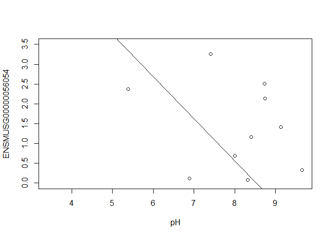
In this case, limma is fitting a linear regression model, which here is a straight line fit, with the slope and intercept defined by the model coefficients:
ENSMUSG00000056054 <- y$E["ENSMUSG00000056054.10",]
plot(ENSMUSG00000056054 ~ pH, ylim = c(0, 3.5))
intercept <- coef(fit)["ENSMUSG00000056054.10", "(Intercept)"]
slope <- coef(fit)["ENSMUSG00000056054.10", "pH"]
abline(a = intercept, b = slope)
slope
## [1] -1.065091
In this example, the log fold change logFC is the slope of the line, or the change in gene expression (on the log2 CPM scale) for each unit increase in pH.
Here, a logFC of 0.20 means a 0.20 log2 CPM increase in gene expression for each unit increase in pH, or a 15% increase on the CPM scale (2^0.20 = 1.15).
A bit more on linear models
Limma fits a linear model to each gene.
Linear models include analysis of variance (ANOVA) models, linear regression, and any model of the form
Y = β0 + β1X1 + β2X2 + … + βpXp + ε
The covariates X can be:
- a continuous variable (pH, HScore score, age, weight, temperature, etc.)
- Dummy variables coding a categorical covariate (like cell type, genotype, and group)
The β’s are unknown parameters to be estimated.
In limma, the β’s are the log fold changes.
The error (residual) term ε is assumed to be normally distributed with a variance that is constant across the range of the data.
Normally distributed means the residuals come from a distribution that looks like this:
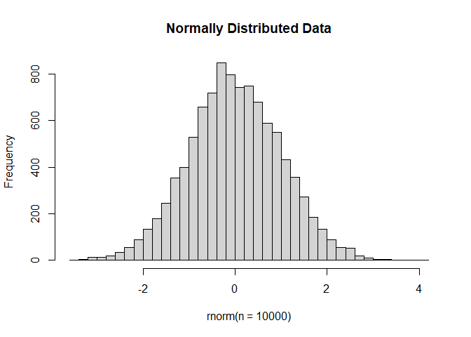
The log2 transformation that voom applies to the counts makes the data “normal enough”, but doesn’t completely stabilize the variance:
mm <- model.matrix(~0 + group + mouse)
tmp <- voom(d, mm, plot = T)
## Coefficients not estimable: mouse206 mouse7531
## Warning: Partial NA coefficients for 16093 probe(s)
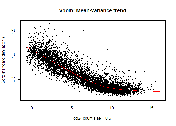
The log2 counts per million are more variable at lower expression levels. The variance weights calculated by voom address this situation.
Both edgeR and limma have VERY comprehensive user manuals
The limma users’ guide has great details on model specification.
Simple plotting
mm <- model.matrix(~genotype*cell_type + mouse)
colnames(mm) <- make.names(colnames(mm))
y <- voom(d, mm, plot = F)
## Coefficients not estimable: mouse206 mouse7531
## Warning: Partial NA coefficients for 16093 probe(s)
fit <- lmFit(y, mm)
## Coefficients not estimable: mouse206 mouse7531
## Warning: Partial NA coefficients for 16093 probe(s)
contrast.matrix <- makeContrasts(genotypeKOMIR150, levels=colnames(coef(fit)))
fit2 <- contrasts.fit(fit, contrast.matrix)
fit2 <- eBayes(fit2)
top.table <- topTable(fit2, coef = 1, sort.by = "P", n = 40)
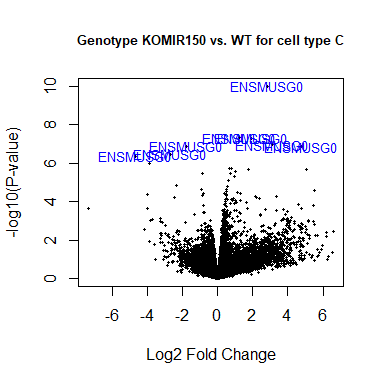
Volcano plot
volcanoplot(fit2, coef=1, highlight=8, names=rownames(fit2), main="Genotype KOMIR150 vs. WT for cell type C", cex.main = 0.8)
head(anno[match(rownames(fit2), anno$Gene.stable.ID.version),
     c("Gene.stable.ID.version", "Gene.name") ])
##        Gene.stable.ID.version Gene.name
## 101955   ENSMUSG00000098104.2    Gm6085
## 102117  ENSMUSG00000033845.14    Mrpl15
## 102222   ENSMUSG00000102275.2   Gm37144
## 102893  ENSMUSG00000025903.15    Lypla1
## 103351  ENSMUSG00000033813.16     Tcea1
## 105668  ENSMUSG00000033793.13   Atp6v1h
identical(anno[match(rownames(fit2), anno$Gene.stable.ID.version),
     c("Gene.stable.ID.version")], rownames(fit2))
## [1] TRUE
volcanoplot(fit2, coef=1, highlight=8, names=anno[match(rownames(fit2), anno$Gene.stable.ID.version), "Gene.name"], main="Genotype KOMIR150 vs. WT for cell type C", cex.main = 0.8)

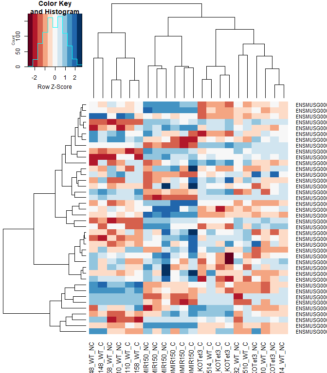
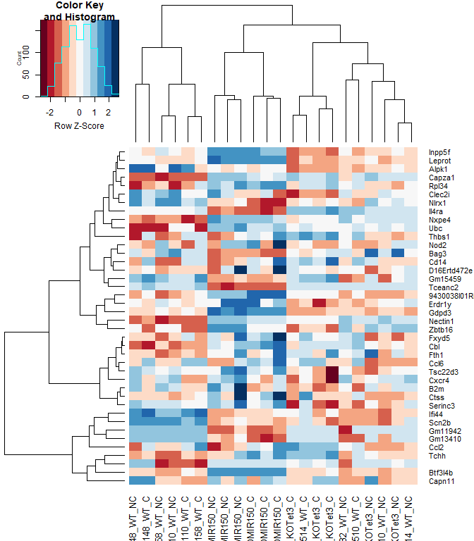
Heatmap
#using a red and blue color scheme without traces and scaling each row
heatmap.2(logcpm[rownames(top.table),],col=brewer.pal(11,"RdBu"),scale="row", trace="none")
anno[match(rownames(top.table), anno$Gene.stable.ID.version),
     c("Gene.stable.ID.version", "Gene.name")]
##        Gene.stable.ID.version     Gene.name
## 133968   ENSMUSG00000030703.9         Gdpd3
## 67174   ENSMUSG00000008348.10           Ubc
## 7220     ENSMUSG00000066687.6        Zbtb16
## 85232   ENSMUSG00000044229.10         Nxpe4
## 117746  ENSMUSG00000030748.10         Il4ra
## 42355   ENSMUSG00000032012.10       Nectin1
## 13240   ENSMUSG00000028619.16       Tceanc2
## 5616    ENSMUSG00000028037.14         Ifi44
## 95589    ENSMUSG00000094344.2       Gm11942
## 74077   ENSMUSG00000070372.12        Capza1
## 79718   ENSMUSG00000035212.15        Leprot
## 2748    ENSMUSG00000096768.10        Erdr1y
## 94729    ENSMUSG00000121395.1
## 45713   ENSMUSG00000055994.16          Nod2
## 35574   ENSMUSG00000028028.12         Alpk1
## 144729  ENSMUSG00000042105.19        Inpp5f
## 48373    ENSMUSG00000045382.7         Cxcr4
## 32313   ENSMUSG00000031431.14       Tsc22d3
## 19148    ENSMUSG00000100801.2       Gm15459
## 47875   ENSMUSG00000034342.10           Cbl
## 102611  ENSMUSG00000009687.15         Fxyd5
## 113132  ENSMUSG00000030365.12        Clec2i
## 95065   ENSMUSG00000058626.17        Capn11
## 39722   ENSMUSG00000062006.13         Rpl34
## 144811  ENSMUSG00000040139.15 9430038I01Rik
## 96938   ENSMUSG00000017707.10       Serinc3
## 144725   ENSMUSG00000030847.9          Bag3
## 72576    ENSMUSG00000051439.8          Cd14
## 102581  ENSMUSG00000038642.11          Ctss
## 141086   ENSMUSG00000083116.2       Gm13410
## 49014   ENSMUSG00000032109.16         Nlrx1
## 35112    ENSMUSG00000024661.8          Fth1
## 65556    ENSMUSG00000114133.2       Btf3l4b
## 131385   ENSMUSG00000040152.9         Thbs1
## 95219    ENSMUSG00000052415.6          Tchh
## 127160  ENSMUSG00000070304.14         Scn2b
## 66102    ENSMUSG00000060802.9           B2m
## 143801   ENSMUSG00000035385.6          Ccl2
## 34447   ENSMUSG00000022864.15   D16Ertd472e
## 132646   ENSMUSG00000018927.4          Ccl6
identical(anno[match(rownames(top.table), anno$Gene.stable.ID.version), "Gene.stable.ID.version"], rownames(top.table))
## [1] TRUE
heatmap.2(logcpm[rownames(top.table),],col=brewer.pal(11,"RdBu"),scale="row", trace="none", labRow = anno[match(rownames(top.table), anno$Gene.stable.ID.version), "Gene.name"])
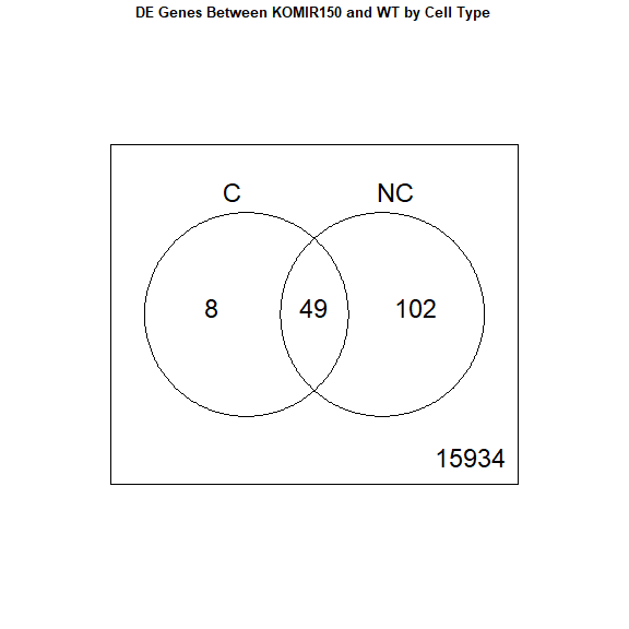
2 factor venn diagram
mm <- model.matrix(~genotype*cell_type + mouse)
colnames(mm) <- make.names(colnames(mm))
y <- voom(d, mm, plot = F)
## Coefficients not estimable: mouse206 mouse7531
## Warning: Partial NA coefficients for 16093 probe(s)
fit <- lmFit(y, mm)
## Coefficients not estimable: mouse206 mouse7531
## Warning: Partial NA coefficients for 16093 probe(s)
contrast.matrix <- makeContrasts(genotypeKOMIR150, genotypeKOMIR150 + genotypeKOMIR150.cell_typeNC, levels=colnames(coef(fit)))
fit2 <- contrasts.fit(fit, contrast.matrix)
fit2 <- eBayes(fit2)
top.table <- topTable(fit2, coef = 1, sort.by = "P", n = 40)

results <- decideTests(fit2)
vennDiagram(results, names = c("C", "NC"), main = "DE Genes Between KOMIR150 and WT by Cell Type", cex.main = 0.8)
Download the Enrichment Analysis R Markdown document
download.file("https://raw.githubusercontent.com/ucdavis-bioinformatics-training/2023-June-RNA-Seq-Analysis/master/data_analysis/enrichment_mm.Rmd", "enrichment_mm.Rmd")
sessionInfo()
## R version 4.4.0 (2024-04-24 ucrt)
## Platform: x86_64-w64-mingw32/x64
## Running under: Windows 10 x64 (build 19045)
##
## Matrix products: default
##
##
## locale:
## [1] LC_COLLATE=English_United States.utf8
## [2] LC_CTYPE=English_United States.utf8
## [3] LC_MONETARY=English_United States.utf8
## [4] LC_NUMERIC=C
## [5] LC_TIME=English_United States.utf8
##
## time zone: America/Los_Angeles
## tzcode source: internal
##
## attached base packages:
## [1] stats     graphics  grDevices utils     datasets  methods   base
##
## other attached packages:
## [1] gplots_3.1.3.1     RColorBrewer_1.1-3 edgeR_4.2.0        limma_3.60.3
##
## loaded via a namespace (and not attached):
##  [1] cli_3.6.3          knitr_1.47         rlang_1.1.4        xfun_0.45
##  [5] highr_0.11         KernSmooth_2.23-22 jsonlite_1.8.8     gtools_3.9.5
##  [9] statmod_1.5.0      htmltools_0.5.8.1  sass_0.4.9         locfit_1.5-9.10
## [13] rmarkdown_2.27     grid_4.4.0         evaluate_0.24.0    jquerylib_0.1.4
## [17] caTools_1.18.2     bitops_1.0-7       fastmap_1.2.0      yaml_2.3.8
## [21] lifecycle_1.0.4    compiler_4.4.0     Rcpp_1.0.12        rstudioapi_0.16.0
## [25] lattice_0.22-6     digest_0.6.35      R6_2.5.1           bslib_0.7.0
## [29] tools_4.4.0        cachem_1.1.0