
GO AND KEGG Enrichment Analysis
Load libraries
library(topGO)
library(org.Mm.eg.db)
library(clusterProfiler)
library(pathview)
library(enrichplot)
library(ggplot2)
library(dplyr)
Files for examples were created in the DE analysis.
Gene Ontology (GO) Enrichment
Gene ontology provides a controlled vocabulary for describing biological processes (BP ontology), molecular functions (MF ontology) and cellular components (CC ontology)
The GO ontologies themselves are organism-independent; terms are associated with genes for a specific organism through direct experimentation or through sequence homology with another organism and its GO annotation.
Terms are related to other terms through parent-child relationships in a directed acylic graph.
Enrichment analysis provides one way of drawing conclusions about a set of differential expression results.
1. topGO Example Using Kolmogorov-Smirnov Testing Our first example uses Kolmogorov-Smirnov Testing for enrichment testing of our mouse DE results, with GO annotation obtained from the Bioconductor database org.Mm.eg.db.
The first step in each topGO analysis is to create a topGOdata object. This contains the genes, the score for each gene (here we use the p-value from the DE test), the GO terms associated with each gene, and the ontology to be used (here we use the biological process ontology)
infile <- "WT.C_v_WT.NC.txt"
DE <- read.delim(infile)

## Add entrezgene IDs to top table
tmp <- bitr(DE$Gene.stable.ID, fromType = "ENSEMBL", toType = "ENTREZID", OrgDb = org.Mm.eg.db)
## 'select()' returned 1:many mapping between keys and columns
## Warning in bitr(DE$Gene.stable.ID, fromType = "ENSEMBL", toType = "ENTREZID", :
## 15.79% of input gene IDs are fail to map...
id.conv <- subset(tmp, !duplicated(tmp$ENSEMBL))
DE <- left_join(DE, id.conv, by = c("Gene.stable.ID" = "ENSEMBL"))

# Make gene list
DE.nodupENTREZ <- subset(DE, !is.na(ENTREZID) & !duplicated(ENTREZID))
geneList <- DE.nodupENTREZ$P.Value
names(geneList) <- DE.nodupENTREZ$ENTREZID
head(geneList)
##       104718        18795        67241        94212        12521        12772
## 1.705584e-15 2.616034e-15 3.237429e-15 4.128023e-15 4.423061e-15 1.053529e-14
# Create topGOData object
GOdata <- new("topGOdata",
	ontology = "BP",
	allGenes = geneList,
	geneSelectionFun = function(x)x,
	annot = annFUN.org , mapping = "org.Mm.eg.db")
##
## Building most specific GOs .....
## ( 11110 GO terms found. )
##
## Build GO DAG topology ..........
## ( 14385 GO terms and 32270 relations. )
##
## Annotating nodes ...............
## ( 12523 genes annotated to the GO terms. )
2. The topGOdata object is then used as input for enrichment testing:
# Kolmogorov-Smirnov testing
resultKS <- runTest(GOdata, algorithm = "weight01", statistic = "ks")
##
## 			 -- Weight01 Algorithm --
##
## 		 the algorithm is scoring 14385 nontrivial nodes
## 		 parameters:
## 			 test statistic: ks
## 			 score order: increasing
##
## 	 Level 19:	2 nodes to be scored	(0 eliminated genes)
##
## 	 Level 18:	27 nodes to be scored	(0 eliminated genes)
##
## 	 Level 17:	54 nodes to be scored	(33 eliminated genes)
##
## 	 Level 16:	92 nodes to be scored	(102 eliminated genes)
##
## 	 Level 15:	136 nodes to be scored	(217 eliminated genes)
##
## 	 Level 14:	281 nodes to be scored	(502 eliminated genes)
##
## 	 Level 13:	621 nodes to be scored	(840 eliminated genes)
##
## 	 Level 12:	1095 nodes to be scored	(1627 eliminated genes)
##
## 	 Level 11:	1638 nodes to be scored	(2932 eliminated genes)
##
## 	 Level 10:	1941 nodes to be scored	(4979 eliminated genes)
##
## 	 Level 9:	2115 nodes to be scored	(6787 eliminated genes)
##
## 	 Level 8:	2030 nodes to be scored	(8326 eliminated genes)
##
## 	 Level 7:	1810 nodes to be scored	(9479 eliminated genes)
##
## 	 Level 6:	1340 nodes to be scored	(10261 eliminated genes)
##
## 	 Level 5:	718 nodes to be scored	(10777 eliminated genes)
##
## 	 Level 4:	350 nodes to be scored	(11069 eliminated genes)
##
## 	 Level 3:	116 nodes to be scored	(11198 eliminated genes)
##
## 	 Level 2:	18 nodes to be scored	(11256 eliminated genes)
##
## 	 Level 1:	1 nodes to be scored	(11288 eliminated genes)
tab <- GenTable(GOdata, raw.p.value = resultKS, topNodes = length(resultKS@score), numChar = 120)
topGO by default preferentially tests more specific terms, utilizing the topology of the GO graph. The algorithms used are described in detail here.
head(tab, 15)
##         GO.ID                                                             Term
## 1  GO:0045071                  negative regulation of viral genome replication
## 2  GO:0045944        positive regulation of transcription by RNA polymerase II
## 3  GO:0032731             positive regulation of interleukin-1 beta production
## 4  GO:0045087                                           innate immune response
## 5  GO:0032760          positive regulation of tumor necrosis factor production
## 6  GO:0051607                                        defense response to virus
## 7  GO:0050830                      defense response to Gram-positive bacterium
## 8  GO:0071285                                 cellular response to lithium ion
## 9  GO:0140972        negative regulation of AIM2 inflammasome complex assembly
## 10 GO:0006002                           fructose 6-phosphate metabolic process
## 11 GO:0032728                positive regulation of interferon-beta production
## 12 GO:0097202               activation of cysteine-type endopeptidase activity
## 13 GO:0051091 positive regulation of DNA-binding transcription factor activity
## 14 GO:0036151                        phosphatidylcholine acyl-chain remodeling
## 15 GO:0072672                                         neutrophil extravasation
##    Annotated Significant Expected raw.p.value
## 1         57          57       57     2.0e-09
## 2        890         890      890     2.9e-09
## 3         61          61       61     7.0e-08
## 4        719         719      719     1.4e-07
## 5        107         107      107     4.3e-07
## 6        263         263      263     1.1e-06
## 7         82          82       82     1.4e-06
## 8         10          10       10     4.3e-06
## 9         12          12       12     4.3e-06
## 10        11          11       11     9.3e-06
## 11        47          47       47     1.7e-05
## 12        24          24       24     1.9e-05
## 13       177         177      177     3.5e-05
## 14         9           9        9     4.6e-05
## 15        15          15       15     4.8e-05
- Annotated: number of genes (in our gene list) that are annotated with the term
- Significant: n/a for this example, same as Annotated here
- Expected: n/a for this example, same as Annotated here
- raw.p.value: P-value from Kolomogorov-Smirnov test that DE p-values annotated with the term are smaller (i.e. more significant) than those not annotated with the term.
The Kolmogorov-Smirnov test directly compares two probability distributions based on their maximum distance.
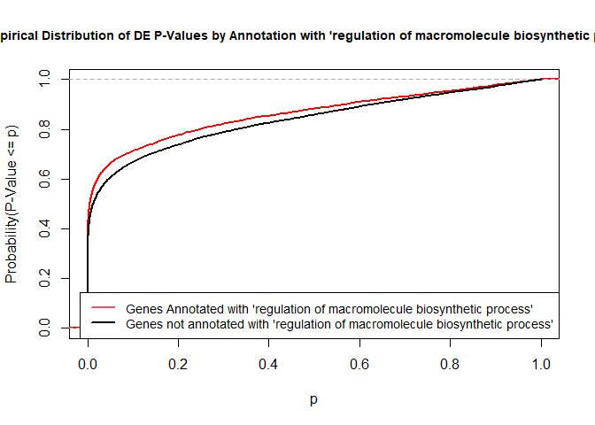
To illustrate the KS test, we plot probability distributions of p-values that are and that are not annotated with the term GO:0010556 “regulation of macromolecule biosynthetic process” (2344 genes) p-value 1.00. (This won’t exactly match what topGO does due to their elimination algorithm):
rna.pp.terms <- genesInTerm(GOdata)[["GO:0010556"]] # get genes associated with term
p.values.in <- geneList[names(geneList) %in% rna.pp.terms]
p.values.out <- geneList[!(names(geneList) %in% rna.pp.terms)]
plot.ecdf(p.values.in, verticals = T, do.points = F, col = "red", lwd = 2, xlim = c(0,1),
          main = "Empirical Distribution of DE P-Values by Annotation with 'regulation of macromolecule biosynthetic process'",
          cex.main = 0.9, xlab = "p", ylab = "Probability(P-Value <= p)")
ecdf.out <- ecdf(p.values.out)
xx <- unique(sort(c(seq(0, 1, length = 201), knots(ecdf.out))))
lines(xx, ecdf.out(xx), col = "black", lwd = 2)
legend("bottomright", legend = c("Genes Annotated with 'regulation of macromolecule biosynthetic process'", "Genes not annotated with 'regulation of macromolecule biosynthetic process'"), lwd = 2, col = 2:1, cex = 0.9)
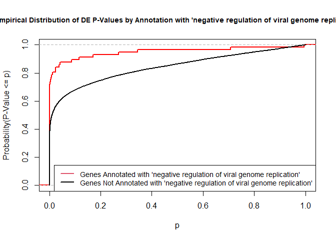
versus the probability distributions of p-values that are and that are not annotated with the term GO:0045071 “negative regulation of viral genome replication” (54 genes) p-value 3.3x10⁻⁹.
rna.pp.terms <- genesInTerm(GOdata)[["GO:0045071"]] # get genes associated with term
p.values.in <- geneList[names(geneList) %in% rna.pp.terms]
p.values.out <- geneList[!(names(geneList) %in% rna.pp.terms)]
plot.ecdf(p.values.in, verticals = T, do.points = F, col = "red", lwd = 2, xlim = c(0,1),
          main = "Empirical Distribution of DE P-Values by Annotation with 'negative regulation of viral genome replication'",
          cex.main = 0.9, xlab = "p", ylab = "Probability(P-Value <= p)")
ecdf.out <- ecdf(p.values.out)
xx <- unique(sort(c(seq(0, 1, length = 201), knots(ecdf.out))))
lines(xx, ecdf.out(xx), col = "black", lwd = 2)
legend("bottomright", legend = c("Genes Annotated with 'negative regulation of viral genome replication'", "Genes Not Annotated with 'negative regulation of viral genome replication'"), lwd = 2, col = 2:1, cex = 0.9)
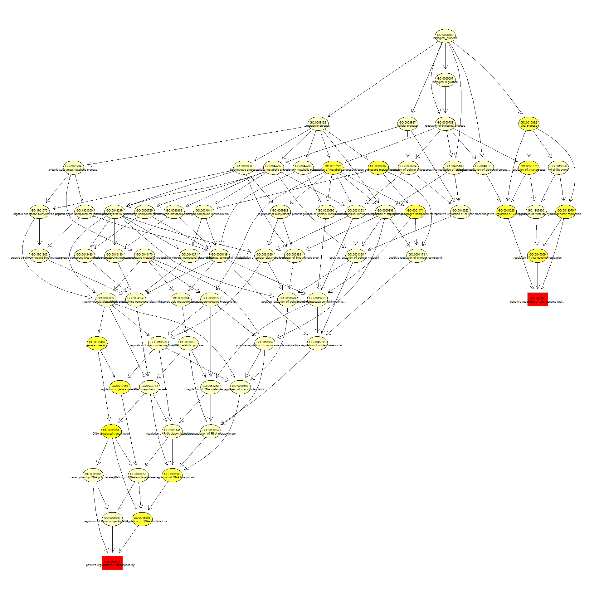
We can use the function showSigOfNodes to plot the GO graph for the 2 most significant terms and their parents, color coded by enrichment p-value (red is most significant):
par(cex = 0.3)
showSigOfNodes(GOdata, score(resultKS), firstSigNodes = 2, useInfo = "def", .NO.CHAR = 40)
## Loading required package: Rgraphviz
## Loading required package: grid
##
## Attaching package: 'grid'
## The following object is masked from 'package:topGO':
##
##     depth
##
## Attaching package: 'Rgraphviz'
## The following objects are masked from 'package:IRanges':
##
##     from, to
## The following objects are masked from 'package:S4Vectors':
##
##     from, to
## $dag
## A graphNEL graph with directed edges
## Number of Nodes = 68
## Number of Edges = 155
##
## $complete.dag
## [1] "A graph with 68 nodes."
par(cex = 1)
3. topGO Example Using Fisher’s Exact Test
Next, we use Fisher’s exact test to test for GO enrichment among significantly DE genes.
Create topGOdata object:
geneList <- DE.nodupENTREZ$adj.P.Val
names(geneList) <- DE.nodupENTREZ$ENTREZID

# Create topGOData object
GOdata <- new("topGOdata",
	ontology = "BP",
	allGenes = geneList,
	geneSelectionFun = function(x) (x < 0.05),
	annot = annFUN.org , mapping = "org.Mm.eg.db")
##
## Building most specific GOs .....
## ( 11110 GO terms found. )
##
## Build GO DAG topology ..........
## ( 14385 GO terms and 32270 relations. )
##
## Annotating nodes ...............
## ( 12523 genes annotated to the GO terms. )
Run Fisher’s Exact Test:
resultFisher <- runTest(GOdata, algorithm = "elim", statistic = "fisher")
##
## 			 -- Elim Algorithm --
##
## 		 the algorithm is scoring 13091 nontrivial nodes
## 		 parameters:
## 			 test statistic: fisher
## 			 cutOff: 0.01
##
## 	 Level 19:	2 nodes to be scored	(0 eliminated genes)
##
## 	 Level 18:	23 nodes to be scored	(0 eliminated genes)
##
## 	 Level 17:	46 nodes to be scored	(12 eliminated genes)
##
## 	 Level 16:	82 nodes to be scored	(22 eliminated genes)
##
## 	 Level 15:	116 nodes to be scored	(77 eliminated genes)
##
## 	 Level 14:	244 nodes to be scored	(102 eliminated genes)
##
## 	 Level 13:	536 nodes to be scored	(277 eliminated genes)
##
## 	 Level 12:	973 nodes to be scored	(538 eliminated genes)
##
## 	 Level 11:	1460 nodes to be scored	(2064 eliminated genes)
##
## 	 Level 10:	1760 nodes to be scored	(2215 eliminated genes)
##
## 	 Level 9:	1924 nodes to be scored	(3237 eliminated genes)
##
## 	 Level 8:	1879 nodes to be scored	(3919 eliminated genes)
##
## 	 Level 7:	1659 nodes to be scored	(4558 eliminated genes)
##
## 	 Level 6:	1246 nodes to be scored	(5649 eliminated genes)
##
## 	 Level 5:	678 nodes to be scored	(6209 eliminated genes)
##
## 	 Level 4:	334 nodes to be scored	(7481 eliminated genes)
##
## 	 Level 3:	110 nodes to be scored	(8857 eliminated genes)
##
## 	 Level 2:	18 nodes to be scored	(8857 eliminated genes)
##
## 	 Level 1:	1 nodes to be scored	(10926 eliminated genes)
tab <- GenTable(GOdata, raw.p.value = resultFisher, topNodes = length(resultFisher@score),
				numChar = 120)
head(tab)
##        GO.ID                                                               Term
## 1 GO:0032731               positive regulation of interleukin-1 beta production
## 2 GO:0045944          positive regulation of transcription by RNA polymerase II
## 3 GO:1901224 positive regulation of non-canonical NF-kappaB signal transduction
## 4 GO:0001525                                                       angiogenesis
## 5 GO:0051607                                          defense response to virus
## 6 GO:0042742                                      defense response to bacterium
##   Annotated Significant Expected raw.p.value
## 1        61          53    35.90     1.8e-06
## 2       890         589   523.85     2.0e-06
## 3        54          47    31.78     6.5e-06
## 4       381         272   224.26     6.6e-06
## 5       263         193   154.80     1.9e-05
## 6       206         154   121.25     2.1e-05
- Annotated: number of genes (in our gene list) that are annotated with the term
- Significant: Number of significantly DE genes annotated with that term (i.e. genes where geneList = 1)
- Expected: Under random chance, number of genes that would be expected to be significantly DE and annotated with that term
- raw.p.value: P-value from Fisher’s Exact Test, testing for association between significance and pathway membership.
Fisher’s Exact Test is applied to the table:
| Significance/Annotation | Annotated With GO Term | Not Annotated With GO Term |
|---|---|---|
| Significantly DE | n1 | n3 |
| Not Significantly DE | n2 | n4 |
and compares the probability of the observed table, conditional on the row and column sums, to what would be expected under random chance.
Advantages over KS (or Wilcoxon) Tests:
-
Ease of interpretation
-
Can be applied when you just have a gene list without associated p-values, etc.
Disadvantages:
- Relies on significant/non-significant dichotomy (an interesting gene could have an adjusted p-value of 0.051 and be counted as non-significant)
- Less powerful
- May be less useful if there are very few (or a large number of) significant genes
Quiz 1
KEGG Pathway Enrichment Testing With clusterProfiler
KEGG, the Kyoto Encyclopedia of Genes and Genomes (https://www.genome.jp/kegg/), provides assignment of genes for many organisms into pathways.
We will conduct KEGG enrichment testing using the Bioconductor package clusterProfiler. clusterProfiler implements an algorithm very similar to that used by GSEA.
Cluster profiler can do much more than KEGG enrichment, check out the clusterProfiler book.
We will base our KEGG enrichment analysis on the t statistics from differential expression, which allows for directional testing.
geneList.KEGG <- DE.nodupENTREZ$t
geneList.KEGG <- sort(geneList.KEGG, decreasing = TRUE)
names(geneList.KEGG) <- DE.nodupENTREZ$ENTREZID
head(geneList.KEGG)
##   104718    18795    67241    94212    12521    12772
## 46.30958 41.37645 40.66526 36.61842 36.45324 36.41880
set.seed(99)
KEGG.results <- gseKEGG(gene = geneList.KEGG, organism = "mmu", pvalueCutoff = 1)
## Reading KEGG annotation online: "https://rest.kegg.jp/link/mmu/pathway"...
## Reading KEGG annotation online: "https://rest.kegg.jp/list/pathway/mmu"...
## using 'fgsea' for GSEA analysis, please cite Korotkevich et al (2019).
## preparing geneSet collections...
## GSEA analysis...
## leading edge analysis...
## done...
KEGG.results <- setReadable(KEGG.results, OrgDb = "org.Mm.eg.db", keyType = "ENTREZID")
outdat <- as.data.frame(KEGG.results)
head(outdat)
##                ID
## mmu05200 mmu05200
## mmu05165 mmu05165
## mmu04970 mmu04970
## mmu04961 mmu04961
## mmu04015 mmu04015
## mmu05160 mmu05160
##                                                                                     Description
## mmu05200                                        Pathways in cancer - Mus musculus (house mouse)
## mmu05165                            Human papillomavirus infection - Mus musculus (house mouse)
## mmu04970                                        Salivary secretion - Mus musculus (house mouse)
## mmu04961 Endocrine and other factor-regulated calcium reabsorption - Mus musculus (house mouse)
## mmu04015                                    Rap1 signaling pathway - Mus musculus (house mouse)
## mmu05160                                               Hepatitis C - Mus musculus (house mouse)
##          setSize enrichmentScore      NES       pvalue     p.adjust
## mmu05200     383       0.3775237 1.706969 1.247349e-07 4.128726e-05
## mmu05165     243       0.4007015 1.736567 1.902410e-06 3.148489e-04
## mmu04970      47       0.6289045 2.105886 4.779633e-06 5.273529e-04
## mmu04961      34       0.6843389 2.164339 6.445738e-06 5.333848e-04
## mmu04015     156       0.4494154 1.849634 8.060359e-06 5.335958e-04
## mmu05160     122       0.4685525 1.882945 1.117934e-05 6.167271e-04
##                qvalue rank                   leading_edge
## mmu05200 2.809818e-05 2374 tags=29%, list=18%, signal=25%
## mmu05165 2.142714e-04 2404 tags=30%, list=18%, signal=26%
## mmu04970 3.588918e-04 1135  tags=34%, list=8%, signal=31%
## mmu04961 3.629968e-04 1164  tags=32%, list=9%, signal=30%
## mmu04015 3.631404e-04 2310 tags=35%, list=17%, signal=29%
## mmu05160 4.197157e-04 2310 tags=41%, list=17%, signal=34%
##                                                                                                                                                                                                                                                                                                                                                                                                                                                                                                                                                                                                                                                             core_enrichment
## mmu05200 Plcb1/Notch1/Pparg/Fn1/Gnaq/Ets1/Cdkn1b/Cebpa/Zbtb16/Met/Fzd7/Jag1/Adcy7/Jup/Rxra/Hes1/Rassf5/Pdgfb/Vegfc/Pten/Raf1/Itgb1/Mgst1/Csf2rb2/Ccnd2/Traf1/Gng2/Rb1/Cxcr4/Mitf/Tcf7l2/Bcl2/Col4a2/Il2rg/Calm1/Arhgef1/Cdh1/Rasgrp2/Apaf1/Il3ra/Bcl2l11/Pld1/Rasgrp1/Tgfbr1/Nfe2l2/Dvl1/Stat2/E2f2/Il6st/Araf/Bad/Cks2/Pdgfrb/Prkcb/Egln3/Casp8/Prkacb/Traf3/Esr1/Brca2/Adcy9/Cdk6/Tgfbr2/Col4a1/Stat5b/Bcr/Map2k1/Nfkb1/Camk2g/Gngt2/Lrp6/Smad3/Stat3/Smo/Fas/Ralb/Jak2/Pik3cd/Kras/Akt3/Pik3r2/Hgf/Itgav/Spi1/Pim2/Nfkbia/Crk/Tfg/Akt1/Gadd45g/Mgst3/Calml4/Elk1/Csf1r/Egln2/Il15/Ednrb/Traf2/Gnb1/Sp1/Ppard/Mlh1/Fgfr1/Itga3/Lpar4/Keap1/Chuk/Mapk3/Gng10/Ptger4/Txnrd1
## mmu05165                                                                                                                                                                                                        Notch1/Fn1/Itga1/H2-Q6/Cdkn1b/Fzd7/Jag1/Hes1/Pten/Raf1/Itgb1/Atp6v1b2/Ccnd2/Atp6v1a/Tbpl1/Rb1/Tcf7l2/Thbs1/Col4a2/Vwf/H2-K1/Tyk2/Isg15/Scrib/Maml2/Dvl1/Stat2/H2-Q7/Lfng/Ppp2r5c/Atp6v0c/Itga5/Bad/Pdgfrb/Casp8/Prkacb/Traf3/H2-Q4/Cdk6/Eif2ak2/Col4a1/Mx1/H2-T10/Map2k1/Nfkb1/Creb3l2/Fas/H2-D1/Pik3cd/Mx2/Kras/Akt3/Pik3r2/Tcirg1/Ppp2r1b/Itgav/Irf3/Atp6v1g1/Oasl2/Llgl2/Prkci/H2-T24/Akt1/Ikbke/Oasl1/Dlg1/Itga3/Tnf/Chuk/Nfx1/Mapk3/Ptger4/Itgb7/Itgb5
## mmu04970                                                                                                                                                                                                                                                                                                                                                                                                                                                                                                                                                                   Plcb1/Gnaq/Adrb1/Adcy7/Atp2b1/Slc12a2/Atp1a1/Bst1/Calm1/Adrb2/Lyz2/Itpr1/Prkcb/Cst3/Prkacb/Adcy9
## mmu04961                                                                                                                                                                                                                                                                                                                                                                                                                                                                                                                                                                                                   Plcb1/Gnaq/Ap2a2/Atp2b1/Atp1a1/Clta/Prkcb/Prkacb/Esr1/Adcy9/Cltb
## mmu04015                                                                                                                                                                                                                                                                                                                                     Plcb1/Sipa1l1/Gnaq/Met/Adcy7/P2ry1/Tiam1/Rassf5/Pdgfb/Vegfc/Raf1/Itgb1/Afdn/Itgal/Fpr1/Insr/Vasp/Prkd2/Thbs1/Calm1/Evl/Rras/Cdh1/Rasgrp2/Sipa1l3/Rap1b/Rapgef5/Itgb2/Pdgfrb/Prkcb/Adcy9/Rapgef1/Map2k1/Rap1a/Ralb/Pik3cd/Kras/Akt3/Pik3r2/Hgf/Prkci/Crk/Arap3/Akt1/Vav3/Calml4/Csf1r/Rgs14/Apbb1ip/Tln2/Fgfr1/Lcp2/Lpar4/Mapk3
## mmu05160                                                                                                                                                                                                                                                                                                                                                                     Cd81/Rxra/Raf1/Rb1/Nr1h3/Tyk2/Apaf1/Rnasel/Stat2/E2f2/Araf/Bad/Eif2ak4/Rsad2/Casp8/Traf3/Cdk6/Eif2ak2/Cxcl10/Mx1/Ifit1/Map2k1/Nfkb1/Eif3e/Oas1a/Ywhaz/Stat3/Socs3/Fas/Pik3cd/Mx2/Kras/Akt3/Pik3r2/Ppp2r1b/Irf3/Rigi/Nfkbia/Ifit1bl1/Akt1/Ikbke/Cldn20/Oas2/Mavs/Traf2/Irf7/Oas3/Tnf/Chuk/Mapk3
Gene set enrichment analysis output includes the following columns:
-
setSize: Number of genes in pathway
-
enrichmentScore: GSEA enrichment score, a statistic reflecting the degree to which a pathway is overrepresented at the top or bottom of the gene list (the gene list here consists of the t-statistics from the DE test).
-
pvalue: Raw p-value from permutation test of enrichment score
-
p.adjust: Benjamini-Hochberg false discovery rate adjusted p-value
-
qvalue: Storey false discovery rate adjusted p-value
-
rank: Position in ranked list at which maximum enrichment score occurred
-
leading_edge: Statistics from leading edge analysis
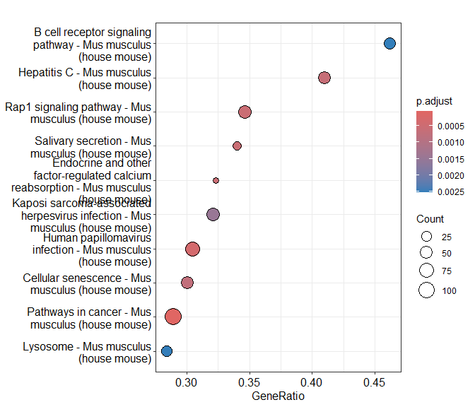
Dotplot of enrichment results
Gene.ratio = (count of core enrichment genes)/(count of pathway genes)
Core enrichment genes = subset of genes that contribute most to the enrichment result (“leading edge subset”)
dotplot(KEGG.results)
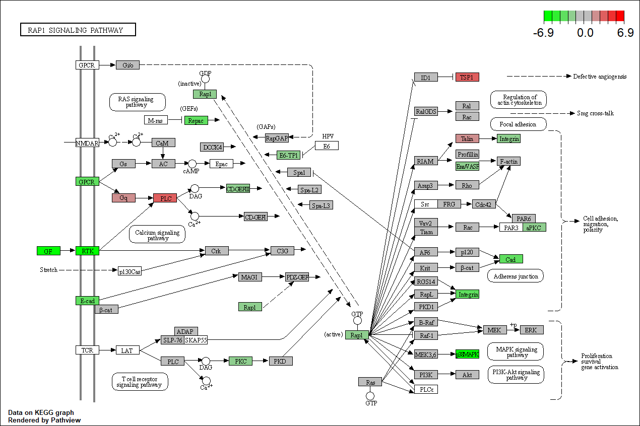
Pathview plot of log fold changes on KEGG diagram
foldChangeList <- DE$logFC
xx <- as.list(org.Mm.egENSEMBL2EG)
names(foldChangeList) <- xx[sapply(strsplit(DE$Gene,split="\\."),"[[", 1L)]
head(foldChangeList)
##    104718     18795     67241     94212     12521     12772
## -2.042255  3.062891 -2.306549 -1.796391 -2.476432  1.972002
mmu04015 <- pathview(gene.data  = foldChangeList,
                     pathway.id = "mmu04015",
                     species    = "mmu",
                     limit      = list(gene=max(abs(foldChangeList)), cpd=1))
## 'select()' returned 1:1 mapping between keys and columns
## Info: Working in directory C:/Users/bpdurbin/OneDrive - University of California, Davis/Desktop/2024-June-RNA-Seq-Analysis/data_analysis
## Info: Writing image file mmu04015.pathview.png
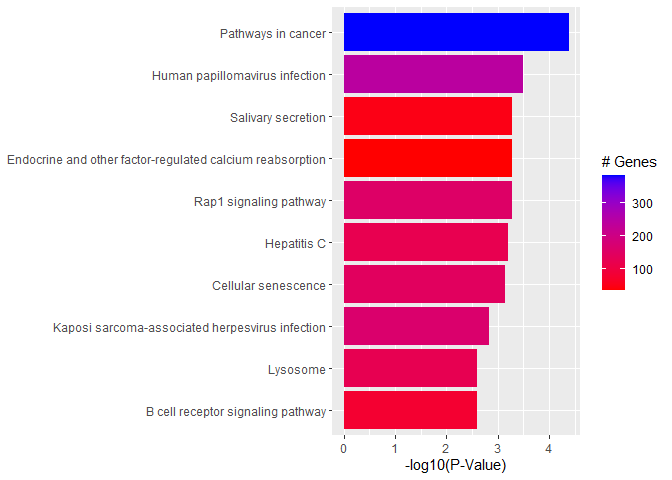
Barplot of p-values for top pathways
A barplot of -log10(p-value) for the top pathways/terms can be used for any type of enrichment analysis.
plotdat <- outdat[1:10,]
plotdat$nice.name <- gsub(" - Mus musculus (house mouse)", "", plotdat$Description, fixed = TRUE)

ggplot(plotdat, aes(x = -log10(p.adjust), y = reorder(nice.name, -log10(p.adjust)), fill = setSize)) + geom_bar(stat = "identity") + labs(x = "-log10(P-Value)", y = NULL, fill = "# Genes") + scale_fill_gradient(low = "red", high = "blue")
Quiz 2
sessionInfo()
## R version 4.4.0 (2024-04-24 ucrt)
## Platform: x86_64-w64-mingw32/x64
## Running under: Windows 10 x64 (build 19045)
##
## Matrix products: default
##
##
## locale:
## [1] LC_COLLATE=English_United States.utf8
## [2] LC_CTYPE=English_United States.utf8
## [3] LC_MONETARY=English_United States.utf8
## [4] LC_NUMERIC=C
## [5] LC_TIME=English_United States.utf8
##
## time zone: America/Los_Angeles
## tzcode source: internal
##
## attached base packages:
## [1] grid      stats4    stats     graphics  grDevices utils     datasets
## [8] methods   base
##
## other attached packages:
##  [1] Rgraphviz_2.48.0       dplyr_1.1.4            ggplot2_3.5.1
##  [4] enrichplot_1.24.0      pathview_1.44.0        clusterProfiler_4.12.0
##  [7] org.Mm.eg.db_3.19.1    topGO_2.56.0           SparseM_1.83
## [10] GO.db_3.19.1           AnnotationDbi_1.66.0   IRanges_2.38.0
## [13] S4Vectors_0.42.0       Biobase_2.64.0         graph_1.82.0
## [16] BiocGenerics_0.50.0
##
## loaded via a namespace (and not attached):
##   [1] RColorBrewer_1.1-3      rstudioapi_0.16.0       jsonlite_1.8.8
##   [4] magrittr_2.0.3          farver_2.1.2            rmarkdown_2.27
##   [7] fs_1.6.4                zlibbioc_1.50.0         vctrs_0.6.5
##  [10] memoise_2.0.1           RCurl_1.98-1.14         ggtree_3.12.0
##  [13] htmltools_0.5.8.1       gridGraphics_0.5-1      sass_0.4.9
##  [16] bslib_0.7.0             plyr_1.8.9              cachem_1.1.0
##  [19] igraph_2.0.3            lifecycle_1.0.4         pkgconfig_2.0.3
##  [22] Matrix_1.7-0            R6_2.5.1                fastmap_1.2.0
##  [25] gson_0.1.0              GenomeInfoDbData_1.2.12 digest_0.6.35
##  [28] aplot_0.2.3             colorspace_2.1-0        patchwork_1.2.0
##  [31] RSQLite_2.3.7           org.Hs.eg.db_3.19.1     labeling_0.4.3
##  [34] fansi_1.0.6             httr_1.4.7              polyclip_1.10-6
##  [37] compiler_4.4.0          bit64_4.0.5             withr_3.0.0
##  [40] BiocParallel_1.38.0     viridis_0.6.5           DBI_1.2.3
##  [43] highr_0.11              ggforce_0.4.2           MASS_7.3-60.2
##  [46] HDO.db_0.99.1           tools_4.4.0             ape_5.8
##  [49] scatterpie_0.2.3        glue_1.7.0              nlme_3.1-164
##  [52] GOSemSim_2.30.0         shadowtext_0.1.3        reshape2_1.4.4
##  [55] snow_0.4-4              fgsea_1.30.0            generics_0.1.3
##  [58] gtable_0.3.5            tidyr_1.3.1             data.table_1.15.4
##  [61] tidygraph_1.3.1         utf8_1.2.4              XVector_0.44.0
##  [64] ggrepel_0.9.5           pillar_1.9.0            stringr_1.5.1
##  [67] yulab.utils_0.1.4       splines_4.4.0           tweenr_2.0.3
##  [70] treeio_1.28.0           lattice_0.22-6          bit_4.0.5
##  [73] tidyselect_1.2.1        Biostrings_2.72.1       knitr_1.47
##  [76] gridExtra_2.3           xfun_0.45               graphlayouts_1.1.1
##  [79] matrixStats_1.3.0       KEGGgraph_1.64.0        stringi_1.8.4
##  [82] UCSC.utils_1.0.0        lazyeval_0.2.2          ggfun_0.1.5
##  [85] yaml_2.3.8              evaluate_0.24.0         codetools_0.2-20
##  [88] ggraph_2.2.1            tibble_3.2.1            qvalue_2.36.0
##  [91] ggplotify_0.1.2         cli_3.6.3               munsell_0.5.1
##  [94] jquerylib_0.1.4         Rcpp_1.0.12             GenomeInfoDb_1.40.1
##  [97] png_0.1-8               XML_3.99-0.16.1         parallel_4.4.0
## [100] blob_1.2.4              DOSE_3.30.1             bitops_1.0-7
## [103] viridisLite_0.4.2       tidytree_0.4.6          scales_1.3.0
## [106] purrr_1.0.2             crayon_1.5.3            rlang_1.1.4
## [109] cowplot_1.1.3           fastmatch_1.1-4         KEGGREST_1.44.1