
Load libraries
library(topGO)
library(org.Mm.eg.db)
library(clusterProfiler)
library(pathview)
library(enrichplot)
library(ggplot2)
library(dplyr)
Files for examples were created in the DE analysis.
Gene Ontology (GO) Enrichment
Gene ontology provides a controlled vocabulary for describing biological processes (BP ontology), molecular functions (MF ontology) and cellular components (CC ontology)
The GO ontologies themselves are organism-independent; terms are associated with genes for a specific organism through direct experimentation or through sequence homology with another organism and its GO annotation.
Terms are related to other terms through parent-child relationships in a directed acylic graph.
Enrichment analysis provides one way of drawing conclusions about a set of differential expression results.
1. topGO Example Using Kolmogorov-Smirnov Testing Our first example uses Kolmogorov-Smirnov Testing for enrichment testing of our mouse DE results, with GO annotation obtained from the Bioconductor database org.Mm.eg.db.
The first step in each topGO analysis is to create a topGOdata object. This contains the genes, the score for each gene (here we use the p-value from the DE test), the GO terms associated with each gene, and the ontology to be used (here we use the biological process ontology)
infile <- "WT.C_v_WT.NC.txt"
DE <- read.delim(infile)

## Add entrezgene IDs to top table
tmp <- bitr(DE$Gene.stable.ID, fromType = "ENSEMBL", toType = "ENTREZID", OrgDb = org.Mm.eg.db)
## 'select()' returned 1:many mapping between keys and columns
## Warning in bitr(DE$Gene.stable.ID, fromType = "ENSEMBL", toType = "ENTREZID", :
## 20.42% of input gene IDs are fail to map...
id.conv <- subset(tmp, !duplicated(tmp$ENSEMBL))
DE <- left_join(DE, id.conv, by = c("Gene.stable.ID" = "ENSEMBL"))

# Make gene list
DE.nodupENTREZ <- subset(DE, !is.na(ENTREZID) & !duplicated(ENTREZID))
geneList <- DE.nodupENTREZ$P.Value
names(geneList) <- DE.nodupENTREZ$ENTREZID
head(geneList)
##        67241        18795       104718        12521        94212        12772
## 4.109222e-16 7.877908e-16 1.094372e-15 2.224431e-15 2.256262e-15 2.467758e-15
# Create topGOData object
GOdata <- new("topGOdata",
	ontology = "BP",
	allGenes = geneList,
	geneSelectionFun = function(x)x,
	annot = annFUN.org , mapping = "org.Mm.eg.db")
##
## Building most specific GOs .....
## ( 11080 GO terms found. )
##
## Build GO DAG topology ..........
## ( 14033 GO terms and 30925 relations. )
##
## Annotating nodes ...............
## ( 12273 genes annotated to the GO terms. )
2. The topGOdata object is then used as input for enrichment testing:
# Kolmogorov-Smirnov testing
resultKS <- runTest(GOdata, algorithm = "weight01", statistic = "ks")
##
## 			 -- Weight01 Algorithm --
##
## 		 the algorithm is scoring 14033 nontrivial nodes
## 		 parameters:
## 			 test statistic: ks
## 			 score order: increasing
##
## 	 Level 19:	2 nodes to be scored	(0 eliminated genes)
##
## 	 Level 18:	27 nodes to be scored	(0 eliminated genes)
##
## 	 Level 17:	57 nodes to be scored	(46 eliminated genes)
##
## 	 Level 16:	100 nodes to be scored	(115 eliminated genes)
##
## 	 Level 15:	141 nodes to be scored	(239 eliminated genes)
##
## 	 Level 14:	255 nodes to be scored	(587 eliminated genes)
##
## 	 Level 13:	580 nodes to be scored	(1036 eliminated genes)
##
## 	 Level 12:	1028 nodes to be scored	(1681 eliminated genes)
##
## 	 Level 11:	1568 nodes to be scored	(2913 eliminated genes)
##
## 	 Level 10:	1841 nodes to be scored	(5037 eliminated genes)
##
## 	 Level 9:	2063 nodes to be scored	(6865 eliminated genes)
##
## 	 Level 8:	1936 nodes to be scored	(8367 eliminated genes)
##
## 	 Level 7:	1713 nodes to be scored	(9542 eliminated genes)
##
## 	 Level 6:	1367 nodes to be scored	(10370 eliminated genes)
##
## 	 Level 5:	853 nodes to be scored	(10841 eliminated genes)
##
## 	 Level 4:	383 nodes to be scored	(11167 eliminated genes)
##
## 	 Level 3:	101 nodes to be scored	(11323 eliminated genes)
##
## 	 Level 2:	17 nodes to be scored	(11415 eliminated genes)
##
## 	 Level 1:	1 nodes to be scored	(11449 eliminated genes)
tab <- GenTable(GOdata, raw.p.value = resultKS, topNodes = length(resultKS@score), numChar = 120)
topGO by default preferentially tests more specific terms, utilizing the topology of the GO graph. The algorithms used are described in detail here.
head(tab, 15)
##         GO.ID
## 1  GO:0140242
## 2  GO:0140236
## 3  GO:0002181
## 4  GO:0006002
## 5  GO:0002218
## 6  GO:0045071
## 7  GO:0032760
## 8  GO:0035458
## 9  GO:0050680
## 10 GO:0036151
## 11 GO:0072672
## 12 GO:1901224
## 13 GO:0001525
## 14 GO:0045944
## 15 GO:0042776
##                                                                  Term Annotated
## 1                                          translation at postsynapse        48
## 2                                           translation at presynapse        47
## 3                                             cytoplasmic translation       193
## 4                              fructose 6-phosphate metabolic process        12
## 5                                activation of innate immune response       336
## 6                     negative regulation of viral genome replication        44
## 7             positive regulation of tumor necrosis factor production       102
## 8                                cellular response to interferon-beta        59
## 9                negative regulation of epithelial cell proliferation       110
## 10                          phosphatidylcholine acyl-chain remodeling         9
## 11                                           neutrophil extravasation        15
## 12 positive regulation of non-canonical NF-kappaB signal transduction        52
## 13                                                       angiogenesis       401
## 14          positive regulation of transcription by RNA polymerase II       928
## 15             proton motive force-driven mitochondrial ATP synthesis        64
##    Significant Expected raw.p.value
## 1           48       48     1.3e-08
## 2           47       47     2.5e-08
## 3          193      193     3.3e-07
## 4           12       12     1.8e-06
## 5          336      336     1.9e-06
## 6           44       44     2.5e-06
## 7          102      102     4.3e-06
## 8           59       59     1.1e-05
## 9          110      110     2.2e-05
## 10           9        9     3.0e-05
## 11          15       15     4.3e-05
## 12          52       52     5.2e-05
## 13         401      401     5.5e-05
## 14         928      928     7.5e-05
## 15          64       64     8.5e-05
- Annotated: number of genes (in our gene list) that are annotated with the term
- Significant: n/a for this example, same as Annotated here
- Expected: n/a for this example, same as Annotated here
- raw.p.value: P-value from Kolomogorov-Smirnov test that DE p-values annotated with the term are smaller (i.e. more significant) than those not annotated with the term.
The Kolmogorov-Smirnov test directly compares two probability distributions based on their maximum distance.
To illustrate the KS test, we plot probability distributions of p-values that are and that are not annotated with the term GO:0010556 “regulation of macromolecule biosynthetic process” (2344 genes) p-value 1.00. (This won’t exactly match what topGO does due to their elimination algorithm):
rna.pp.terms <- genesInTerm(GOdata)[["GO:0010556"]] # get genes associated with term
p.values.in <- geneList[names(geneList) %in% rna.pp.terms]
p.values.out <- geneList[!(names(geneList) %in% rna.pp.terms)]
plot.ecdf(p.values.in, verticals = T, do.points = F, col = "red", lwd = 2, xlim = c(0,1),
          main = "Empirical Distribution of DE P-Values\nby Annotation with 'regulation of macromolecule biosynthetic process'",
          cex.main = 0.7, xlab = "p", ylab = "Probability(P-Value <= p)")
ecdf.out <- ecdf(p.values.out)
xx <- unique(sort(c(seq(0, 1, length = 201), knots(ecdf.out))))
lines(xx, ecdf.out(xx), col = "black", lwd = 2)
legend("bottomright", legend = c("Genes Annotated with 'regulation of macromolecule biosynthetic process'", "Genes not annotated with 'regulation of macromolecule biosynthetic process'"), lwd = 2, col = 2:1, cex = 0.7)
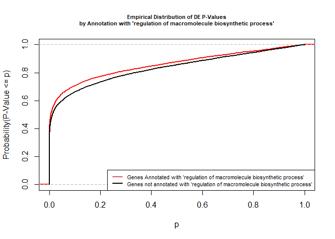
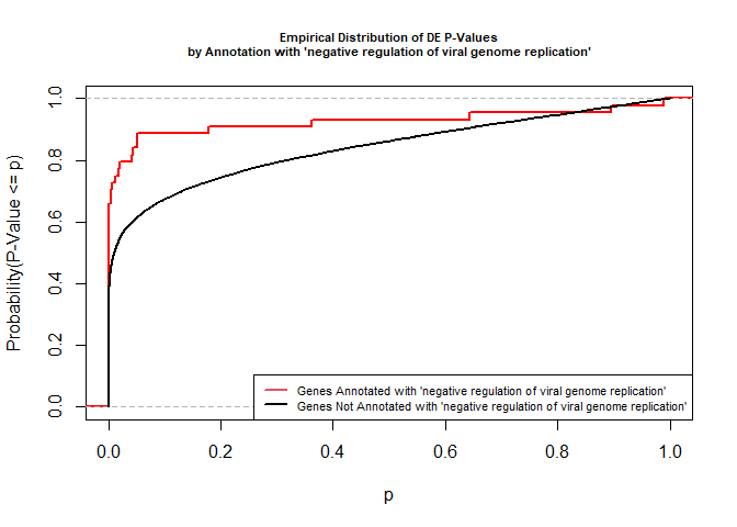
versus the probability distributions of p-values that are and that are not annotated with the term GO:0045071 “negative regulation of viral genome replication” (54 genes) p-value 3.3x10⁻⁹.
rna.pp.terms <- genesInTerm(GOdata)[["GO:0045071"]] # get genes associated with term
p.values.in <- geneList[names(geneList) %in% rna.pp.terms]
p.values.out <- geneList[!(names(geneList) %in% rna.pp.terms)]
plot.ecdf(p.values.in, verticals = T, do.points = F, col = "red", lwd = 2, xlim = c(0,1),
          main = "Empirical Distribution of DE P-Values\nby Annotation with 'negative regulation of viral genome replication'",
          cex.main = 0.7, xlab = "p", ylab = "Probability(P-Value <= p)")
ecdf.out <- ecdf(p.values.out)
xx <- unique(sort(c(seq(0, 1, length = 201), knots(ecdf.out))))
lines(xx, ecdf.out(xx), col = "black", lwd = 2)
legend("bottomright", legend = c("Genes Annotated with 'negative regulation of viral genome replication'", "Genes Not Annotated with 'negative regulation of viral genome replication'"), lwd = 2, col = 2:1, cex = 0.7)
We can use the function showSigOfNodes to plot the GO graph for the 2 most significant terms and their parents, color coded by enrichment p-value (red is most significant):
par(cex = 0.3)
showSigOfNodes(GOdata, score(resultKS), firstSigNodes = 2, useInfo = "def", .NO.CHAR = 40)
## Loading required package: Rgraphviz
## Loading required package: grid
##
## Attaching package: 'grid'
## The following object is masked from 'package:topGO':
##
##     depth
##
## Attaching package: 'Rgraphviz'
## The following objects are masked from 'package:IRanges':
##
##     from, to
## The following objects are masked from 'package:S4Vectors':
##
##     from, to
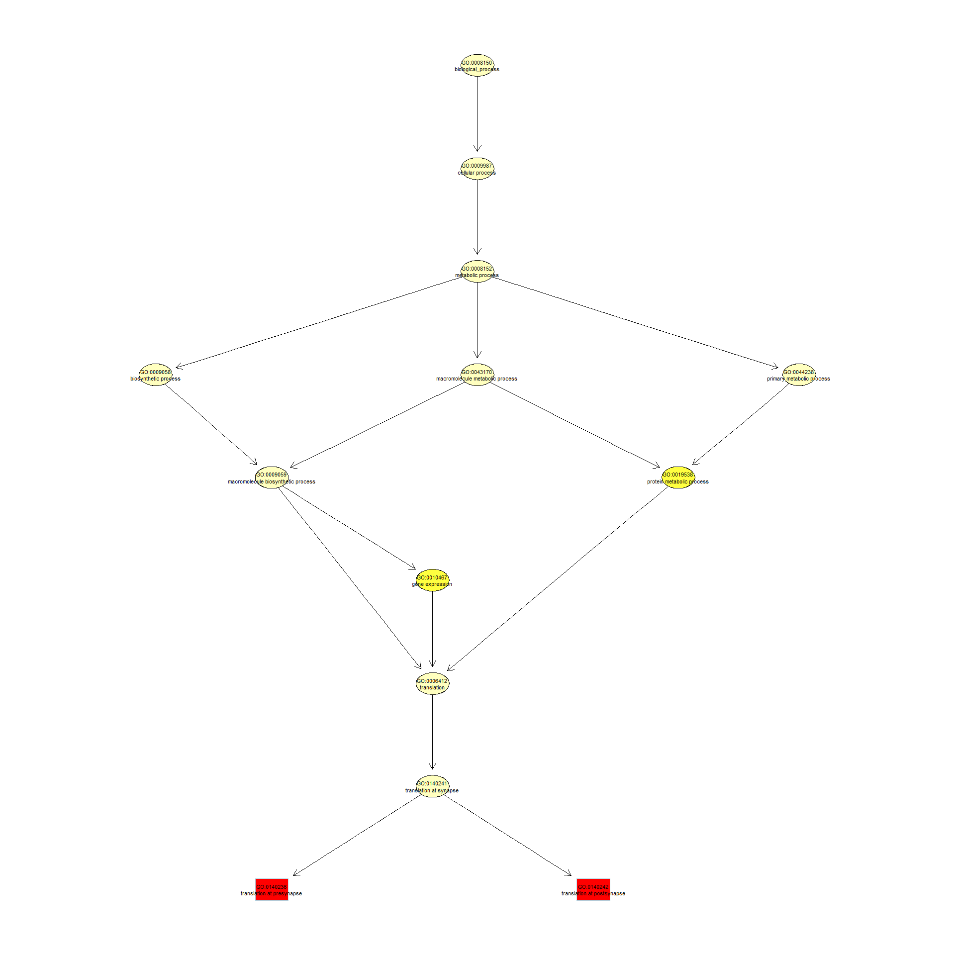
## $dag
## A graphNEL graph with directed edges
## Number of Nodes = 13
## Number of Edges = 16
##
## $complete.dag
## [1] "A graph with 13 nodes."
par(cex = 1)
3. topGO Example Using Fisher’s Exact Test
Next, we use Fisher’s exact test to test for GO enrichment among significantly DE genes.
Create topGOdata object:
geneList <- DE.nodupENTREZ$adj.P.Val
names(geneList) <- DE.nodupENTREZ$ENTREZID

# Create topGOData object
GOdata <- new("topGOdata",
	ontology = "BP",
	allGenes = geneList,
	geneSelectionFun = function(x) (x < 0.05),
	annot = annFUN.org , mapping = "org.Mm.eg.db")
##
## Building most specific GOs .....
## ( 11080 GO terms found. )
##
## Build GO DAG topology ..........
## ( 14033 GO terms and 30925 relations. )
##
## Annotating nodes ...............
## ( 12273 genes annotated to the GO terms. )
Run Fisher’s Exact Test:
resultFisher <- runTest(GOdata, algorithm = "elim", statistic = "fisher")
##
## 			 -- Elim Algorithm --
##
## 		 the algorithm is scoring 12785 nontrivial nodes
## 		 parameters:
## 			 test statistic: fisher
## 			 cutOff: 0.01
##
## 	 Level 19:	2 nodes to be scored	(0 eliminated genes)
##
## 	 Level 18:	22 nodes to be scored	(0 eliminated genes)
##
## 	 Level 17:	50 nodes to be scored	(0 eliminated genes)
##
## 	 Level 16:	90 nodes to be scored	(0 eliminated genes)
##
## 	 Level 15:	121 nodes to be scored	(65 eliminated genes)
##
## 	 Level 14:	213 nodes to be scored	(105 eliminated genes)
##
## 	 Level 13:	492 nodes to be scored	(190 eliminated genes)
##
## 	 Level 12:	913 nodes to be scored	(200 eliminated genes)
##
## 	 Level 11:	1391 nodes to be scored	(1319 eliminated genes)
##
## 	 Level 10:	1670 nodes to be scored	(1602 eliminated genes)
##
## 	 Level 9:	1881 nodes to be scored	(2085 eliminated genes)
##
## 	 Level 8:	1802 nodes to be scored	(2886 eliminated genes)
##
## 	 Level 7:	1578 nodes to be scored	(3988 eliminated genes)
##
## 	 Level 6:	1281 nodes to be scored	(4825 eliminated genes)
##
## 	 Level 5:	794 nodes to be scored	(6015 eliminated genes)
##
## 	 Level 4:	369 nodes to be scored	(6418 eliminated genes)
##
## 	 Level 3:	98 nodes to be scored	(7074 eliminated genes)
##
## 	 Level 2:	17 nodes to be scored	(7158 eliminated genes)
##
## 	 Level 1:	1 nodes to be scored	(7166 eliminated genes)
tab <- GenTable(GOdata, raw.p.value = resultFisher, topNodes = length(resultFisher@score),
				numChar = 120)
head(tab)
##        GO.ID                                 Term Annotated Significant
## 1 GO:0140242           translation at postsynapse        48          44
## 2 GO:0140236            translation at presynapse        47          43
## 3 GO:0002181              cytoplasmic translation       193         144
## 4 GO:0046718        symbiont entry into host cell        72          58
## 5 GO:0001525                         angiogenesis       401         278
## 6 GO:0035458 cellular response to interferon-beta        59          48
##   Expected raw.p.value
## 1    28.35     5.2e-07
## 2    27.76     8.1e-07
## 3   113.98     3.8e-06
## 4    42.52     8.6e-05
## 5   236.82     0.00016
## 6    34.84     0.00022
- Annotated: number of genes (in our gene list) that are annotated with the term
- Significant: Number of significantly DE genes annotated with that term (i.e. genes where geneList = 1)
- Expected: Under random chance, number of genes that would be expected to be significantly DE and annotated with that term
- raw.p.value: P-value from Fisher’s Exact Test, testing for association between significance and pathway membership.
Fisher’s Exact Test is applied to the table:
| Significance/Annotation | Annotated With GO Term | Not Annotated With GO Term |
|---|---|---|
| Significantly DE | n1 | n3 |
| Not Significantly DE | n2 | n4 |
and compares the probability of the observed table, conditional on the row and column sums, to what would be expected under random chance.
Advantages over KS (or Wilcoxon) Tests:
-
Ease of interpretation
-
Can be applied when you just have a gene list without associated p-values, etc.
Disadvantages:
- Relies on significant/non-significant dichotomy (an interesting gene could have an adjusted p-value of 0.051 and be counted as non-significant)
- Less powerful
- May be less useful if there are very few (or a large number of) significant genes
Quiz 1
KEGG Pathway Enrichment Testing With clusterProfiler
KEGG, the Kyoto Encyclopedia of Genes and Genomes (https://www.genome.jp/kegg/), provides assignment of genes for many organisms into pathways.
We will conduct KEGG enrichment testing using the Bioconductor package clusterProfiler. clusterProfiler implements an algorithm very similar to that used by GSEA.
Cluster profiler can do much more than KEGG enrichment, check out the clusterProfiler book.
We will base our KEGG enrichment analysis on the t statistics from differential expression, which allows for directional testing.
geneList.KEGG <- DE.nodupENTREZ$t
geneList.KEGG <- sort(geneList.KEGG, decreasing = TRUE)
names(geneList.KEGG) <- DE.nodupENTREZ$ENTREZID
head(geneList.KEGG)
##    67241    18795   104718    12521    94212    12772
## 46.54613 42.60381 38.54763 37.46686 36.69806 36.23871
set.seed(99)
KEGG.results <- gseKEGG(gene = geneList.KEGG, organism = "mmu", pvalueCutoff = 1)
## Reading KEGG annotation online: "https://rest.kegg.jp/link/mmu/pathway"...
## Reading KEGG annotation online: "https://rest.kegg.jp/list/pathway/mmu"...
## using 'fgsea' for GSEA analysis, please cite Korotkevich et al (2019).
## preparing geneSet collections...
## GSEA analysis...
## leading edge analysis...
## done...
KEGG.results <- setReadable(KEGG.results, OrgDb = "org.Mm.eg.db", keyType = "ENTREZID")
outdat <- as.data.frame(KEGG.results)
head(outdat)
##                ID                                     Description setSize
## mmu05168 mmu05168                Herpes simplex virus 1 infection     161
## mmu04142 mmu04142                             Lysosome biogenesis     229
## mmu04970 mmu04970                              Salivary secretion      47
## mmu04015 mmu04015                          Rap1 signaling pathway     156
## mmu05171 mmu05171                  Coronavirus disease - COVID-19     192
## mmu05167 mmu05167 Kaposi sarcoma-associated herpesvirus infection     165
##          enrichmentScore      NES       pvalue     p.adjust       qvalue rank
## mmu05168       0.4932391 1.969289 1.326900e-07 2.446917e-05 1.436011e-05 2285
## mmu04142       0.4476374 1.871709 1.443609e-07 2.446917e-05 1.436011e-05 2313
## mmu04970       0.6675048 2.204195 3.750326e-07 4.237869e-05 2.487058e-05 1115
## mmu04015       0.4736072 1.890513 7.499323e-07 5.084541e-05 2.983941e-05 2568
## mmu05171       0.4511957 1.844312 7.317951e-07 5.084541e-05 2.983941e-05 3262
## mmu05167       0.4665885 1.875059 1.783696e-06 9.457444e-05 5.550247e-05 3321
##                            leading_edge
## mmu05168 tags=37%, list=17%, signal=31%
## mmu04142 tags=31%, list=17%, signal=26%
## mmu04970  tags=34%, list=8%, signal=31%
## mmu04015 tags=36%, list=19%, signal=30%
## mmu05171 tags=48%, list=24%, signal=37%
## mmu05167 tags=42%, list=24%, signal=33%
##                                                                                                                                                                                                                                                                                                                                                                                                                                                                                                                                            core_enrichment
## mmu05168                                                                                                                                                                                 Pou2f2/C3/H2-Q6/Pilrb2/Ptpn11/Bcl2/Ppp1cb/Daxx/Nxf1/Sp100/Apaf1/Pilra/Tyk2/Ifih1/Sting1/Rnasel/Pilrb1/H2-Q7/Ccl2/H2-K1/Stat2/Itga5/Bad/Bst2/Traf3/Casp8/Tnfsf14/H2-Q4/Hcfc2/H2-T10/Eif2ak2/Oas1a/Tnfrsf14/Fas/H2-Ob/Jak2/Rigi/Eif2b2/Pik3r2/Tlr9/Nfkb1/Socs3/B2m/Oas2/Pik3cd/H2-T24/Tap2/Ikbke/Mavs/H2-D1/Oas3/Nfkbia/Irf3/Akt3/Hcfc1/Irf7/Tapbpl/Tlr2/Chuk/Traf2
## mmu04142                                                                                              Dmxl2/Npc2/Slc29a1/Galns/Lamtor4/Igf2r/Ap2a2/Atp6v1b2/Atp6v1a/Gpr155/Acp2/Ctsc/Mitf/Ctsh/Slc36a1/Lamp2/Ctsb/Slc11a1/Acp5/Glb1/Tpcn2/Hexa/Psap/Clta/Slc29a3/Naga/Asah1/Manba/Ncoa7/Tti1/Atp6v0c/Slc36a4/Lamp1/Gnptab/Borcs6/Scarb2/Laptm4a/Slc15a4/Cltb/Cln3/Npc1/Hexb/Slc17a5/Galc/Gnptg/Arsg/Rraga/Ctsl/Ap5s1/Atp6v1g1/Tlr9/Borcs5/Gla/Vps13c/Slc2a6/Ap2s1/Aga/Vps26b/Tcirg1/Cln5/Clcn7/Hgsnat/Tfeb/Ap3m1/Ctns/Vps16/Wdr7/Kxd1/Lamtor2/Atp6v1d/Tlr7
## mmu04970                                                                                                                                                                                                                                                                                                                                                                                                                                                  Plcb1/Gnaq/Adrb1/Adcy7/Slc12a2/Atp2b1/Bst1/Atp1a1/Adrb2/Calm1/Lyz2/Itpr1/Prkacb/Cst3/Prkcb/Adcy9
## mmu04015                                                                                                                                                                                                         Plcb1/Sipa1l1/Gnaq/P2ry1/Tiam1/Met/Adcy7/Itgb1/Pdgfb/Rassf5/Afdn/Vegfc/Raf1/Itgal/Insr/Fpr1/Prkd2/Thbs1/Vasp/Rasgrp2/Evl/Rras/Cdh1/Calm1/Rap1b/Sipa1l3/Rapgef5/Pdgfrb/Prkcb/Itgb2/Adcy9/Rap1a/Ralb/Map2k1/Pik3r2/Prkci/Calml4/Crk/Pik3cd/Hgf/Rgs14/Kras/Rapgef1/Vav3/Arap3/Tln2/Akt3/Actg1/Fgfr1/Csf1r/Lpar4/Lcp2/Adcy4/Apbb1ip/Akt1/Rac1
## mmu05171 C3/F13a1/Rpl3l/Vwf/Tyk2/C1ra/Isg15/Ifih1/Sting1/Rps9/Nrp1/Ccl2/Rpl28/Rplp0/Stat2/Il6st/C4b/Rpl7a/Rpl41/Ace/Traf3/Mx1/Prkcb/Cxcl10/Eif2ak2/Oas1a/Rpl31/Rpl32/Rpl10a/Rigi/C5ar1/Rpl22/Pik3r2/Mx2/Rpl10/Nfkb1/Oas2/Pik3cd/Rps12/Stat3/Ikbke/Rps26/Mavs/Rpl29/Rps27l/Rpsa/Rps5/Rps18/Rpl13/Rpl14/Oas3/Nfkbia/Irf3/Rpl3/Rpl23a/Rpl15/Nlrp3/Rpl18/Tlr2/Chuk/Rps6/Rpl27a/Tlr7/Rpl11/Rps7/Rps17/Rps28/Rps3/Rps20/Rpl35/Tnf/Rpl37/Fos/Rps4x/Rpl19/Rpl17/Rpl4/Rpl34/Rpl39/Rps27a/Rps2/Rpl6/Rpl36a/Mapk3/Rps15a/Rpl9/Mapk11/Rsl24d1/Rpl13a/Rpl21/Rpl7/Ifnar1
## mmu05167                                                                                                                        C3/H2-Q6/Pik3r6/Ccr1/Nfatc3/Pdgfb/Rcan1/Gng2/Rb1/Raf1/Tcf7l2/Tyk2/E2f2/Calm1/H2-Q7/H2-K1/Itpr1/Stat2/Il6st/Traf3/Casp8/H2-Q4/H2-T10/Eif2ak2/Hck/Fas/Gngt2/Cdk6/Ppp3r1/Jak2/Map2k1/Pik3r2/Cd200r1/Calml4/Nfkb1/Pik3cd/H2-T24/Stat3/Kras/Ikbke/H2-D1/Ppp3ca/Nfkbia/Gng10/Irf3/Akt3/Irf7/Nfatc1/E2f3/Chuk/Traf2/Gng12/Ppp3cb/Akt1/Hif1a/Gnb1/Rac1/Fos/Map2k6/Rps27a/Itpr3/Mapk3/Hras/Mapk11/Ccr3/Angpt2/Cycs/Ifnar1/Ccnd1/Bid
Gene set enrichment analysis output includes the following columns:
-
setSize: Number of genes in pathway
-
enrichmentScore: GSEA enrichment score, a statistic reflecting the degree to which a pathway is overrepresented at the top or bottom of the gene list (the gene list here consists of the t-statistics from the DE test).
-
pvalue: Raw p-value from permutation test of enrichment score
-
p.adjust: Benjamini-Hochberg false discovery rate adjusted p-value
-
qvalue: Storey false discovery rate adjusted p-value
-
rank: Position in ranked list at which maximum enrichment score occurred
-
leading_edge: Statistics from leading edge analysis
Dotplot of enrichment results
Gene.ratio = (count of core enrichment genes)/(count of pathway genes)
Core enrichment genes = subset of genes that contribute most to the enrichment result (“leading edge subset”)
dotplot(KEGG.results)

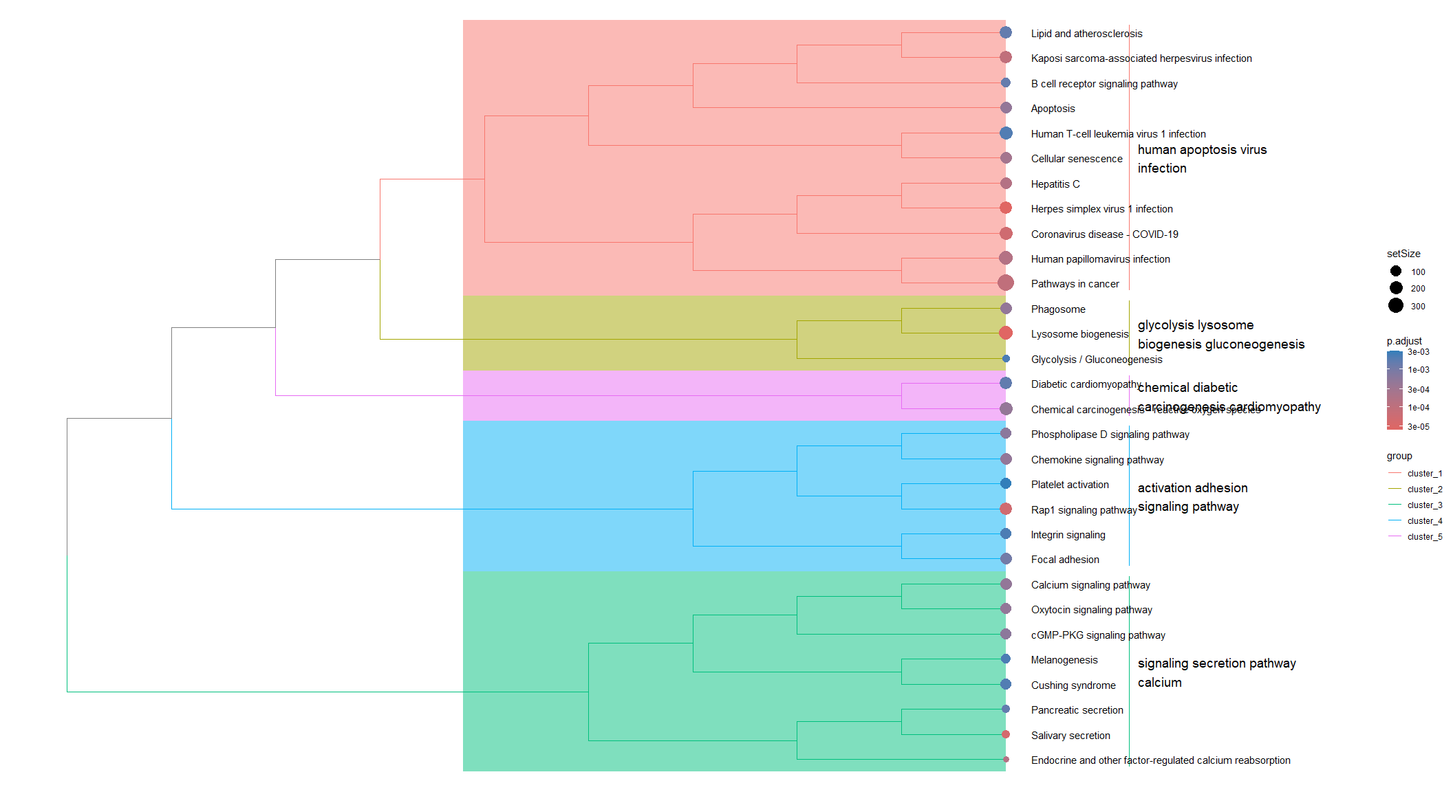
Tree plot of KEGG enrichment
Pathways are clustered based on the degree of overlap in their member genes. Circles are sized based on the number of genes in the pathway and colored based on the adjusted p-value.
tmp <- pairwise_termsim(KEGG.results)
treeplot(tmp, fontsize_cladelab = 5)
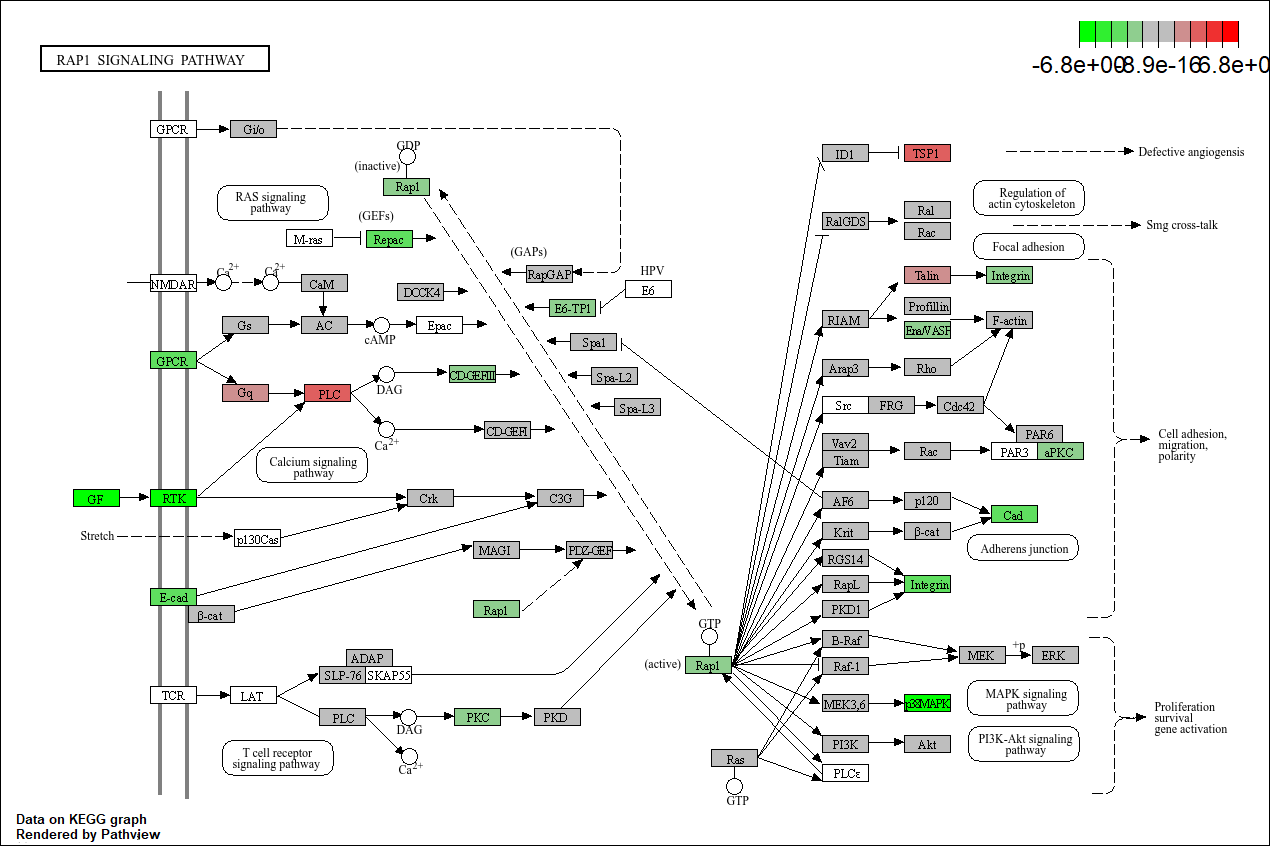
Pathview plot of log fold changes on KEGG diagram
foldChangeList <- DE$logFC
names(foldChangeList) <- DE$ENTREZID
head(foldChangeList)
##     67241     18795    104718     12521     94212     12772
## -2.258712  3.084665 -2.006122 -2.446067 -1.767470  2.024618
mmu04015 <- pathview(gene.data  = foldChangeList,
                     pathway.id = "mmu04015",
                     species    = "mmu",
                     limit      = list(gene = 6))
## 'select()' returned 1:1 mapping between keys and columns
## Info: Working in directory C:/Users/bpdurbin/OneDrive - UC Davis Health/work_stuff/2026-March-RNA-Seq-Analysis/data_analysis
## Info: Writing image file mmu04015.pathview.png
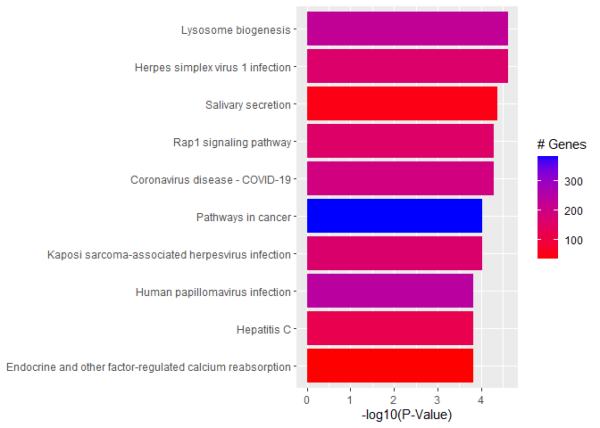
Barplot of p-values for top pathways
A barplot of -log10(p-value) for the top pathways/terms can be used for any type of enrichment analysis.
plotdat <- outdat[1:10,]
plotdat$nice.name <- gsub(" - Mus musculus (house mouse)", "", plotdat$Description, fixed = TRUE)

ggplot(plotdat, aes(x = -log10(p.adjust), y = reorder(nice.name, -log10(p.adjust)), fill = setSize)) + geom_bar(stat = "identity") + labs(x = "-log10(P-Value)", y = NULL, fill = "# Genes") + scale_fill_gradient(low = "red", high = "blue")
Quiz 2
sessionInfo()
## R version 4.5.3 (2026-03-11 ucrt)
## Platform: x86_64-w64-mingw32/x64
## Running under: Windows 11 x64 (build 26100)
##
## Matrix products: default
##   LAPACK version 3.12.1
##
## locale:
## [1] LC_COLLATE=English_United States.utf8
## [2] LC_CTYPE=English_United States.utf8
## [3] LC_MONETARY=English_United States.utf8
## [4] LC_NUMERIC=C
## [5] LC_TIME=English_United States.utf8
##
## time zone: America/Los_Angeles
## tzcode source: internal
##
## attached base packages:
## [1] grid      stats4    stats     graphics  grDevices utils     datasets
## [8] methods   base
##
## other attached packages:
##  [1] Rgraphviz_2.54.0       dplyr_1.2.0            ggplot2_4.0.2
##  [4] enrichplot_1.30.5      pathview_1.31.3        clusterProfiler_4.18.4
##  [7] org.Mm.eg.db_3.22.0    topGO_2.62.0           SparseM_1.84-2
## [10] GO.db_3.22.0           AnnotationDbi_1.72.0   IRanges_2.44.0
## [13] S4Vectors_0.48.0       Biobase_2.70.0         graph_1.88.1
## [16] BiocGenerics_0.56.0    generics_0.1.4
##
## loaded via a namespace (and not attached):
##   [1] RColorBrewer_1.1-3      rstudioapi_0.18.0       jsonlite_2.0.0
##   [4] tidydr_0.0.6            magrittr_2.0.4          ggtangle_0.1.1
##   [7] farver_2.1.2            rmarkdown_2.30          fs_2.0.0
##  [10] vctrs_0.7.2             memoise_2.0.1           RCurl_1.98-1.18
##  [13] ggtree_4.0.5            htmltools_0.5.9         gridGraphics_0.5-1
##  [16] sass_0.4.10             bslib_0.10.0            htmlwidgets_1.6.4
##  [19] plyr_1.8.9              cachem_1.1.0            igraph_2.2.2
##  [22] lifecycle_1.0.5         pkgconfig_2.0.3         Matrix_1.7-5
##  [25] R6_2.6.1                fastmap_1.2.0           gson_0.1.0
##  [28] digest_0.6.39           aplot_0.2.9             ggnewscale_0.5.2
##  [31] patchwork_1.3.2         RSQLite_2.4.6           org.Hs.eg.db_3.22.0
##  [34] labeling_0.4.3          httr_1.4.8              polyclip_1.10-7
##  [37] compiler_4.5.3          bit64_4.6.0-1           fontquiver_0.2.1
##  [40] withr_3.0.2             S7_0.2.1                BiocParallel_1.44.0
##  [43] DBI_1.3.0               ggforce_0.5.0           R.utils_2.13.0
##  [46] MASS_7.3-65             rappdirs_0.3.4          tools_4.5.3
##  [49] otel_0.2.0              ape_5.8-1               scatterpie_0.2.6
##  [52] R.oo_1.27.1             glue_1.8.0              nlme_3.1-168
##  [55] GOSemSim_2.36.0         cluster_2.1.8.2         reshape2_1.4.5
##  [58] fgsea_1.36.2            snow_0.4-4              gtable_0.3.6
##  [61] R.methodsS3_1.8.2       tidyr_1.3.2             data.table_1.18.2.1
##  [64] XVector_0.50.0          ggrepel_0.9.8           pillar_1.11.1
##  [67] stringr_1.6.0           yulab.utils_0.2.4       splines_4.5.3
##  [70] tweenr_2.0.3            treeio_1.34.0           lattice_0.22-9
##  [73] bit_4.6.0               tidyselect_1.2.1        fontLiberation_0.1.0
##  [76] Biostrings_2.78.0       knitr_1.51              fontBitstreamVera_0.1.1
##  [79] Seqinfo_1.0.0           xfun_0.57               matrixStats_1.5.0
##  [82] KEGGgraph_1.70.0        stringi_1.8.7           lazyeval_0.2.2
##  [85] ggfun_0.2.0             yaml_2.3.12             evaluate_1.0.5
##  [88] codetools_0.2-20        gdtools_0.5.0           tibble_3.3.1
##  [91] qvalue_2.42.0           ggplotify_0.1.3         cli_3.6.5
##  [94] systemfonts_1.3.2       jquerylib_0.1.4         Rcpp_1.1.1
##  [97] png_0.1-9               XML_3.99-0.23           parallel_4.5.3
## [100] blob_1.3.0              DOSE_4.4.0              bitops_1.0-9
## [103] tidytree_0.4.7          ggiraph_0.9.6           scales_1.4.0
## [106] purrr_1.2.1             crayon_1.5.3            rlang_1.1.7
## [109] cowplot_1.2.0           fastmatch_1.1-8         KEGGREST_1.50.0