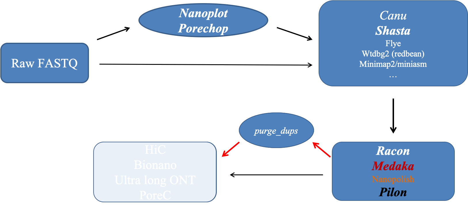
Just a reminder of the overall workflow.

1. Let’s create the working directory and get the raw sequencing data.

First, we are going to get into your own directory and create sub-directories for the raw data.

cd /share/workshop/genome_assembly/$USER

mkdir Nanopore; cd Nanopore
mkdir 00-RawData; cd 00-RawData

Then, let’s get the raw data. We are going to create a soft link to the data in my directory. This way, we can save both disk space and time. There are three sets of data. One is the raw Oxford Nanopore signal data, which were used for basecalling. This set of data would be required if one wants to use nanopolish for polishing the draft assembly, redo the basecall procedure using a different model, or one would like to do any analysis based on the raw signal. Today we are not going to use nanopolish because of run-time concern. Instead, we are going to use medaka, which can produce competitive results comparing to the state-of-the-art signal-based polishing methods. So, we would not use the raw signal data today. It is here so that you know the data is available in general.

ln -s /share/biocore/workshops/Genome-Assembly-Workshop-Jun2020/Nanopore/00-RawData/fast5_pass .

The next piece of data we need to get is the fastq files generated by basecalling, in our case using Guppy 3.0.5, which is based on the flip-flop architecture.

ln -s /share/biocore/workshops/Genome-Assembly-Workshop-Jun2020/Nanopore/00-RawData/fastq_pass .

The third piece of data we need is Illumina sequencing data for polishing using pilon later on.

ln -s /share/biocore/workshops/Genome-Assembly-Workshop-Jun2020/Nanopore/00-RawData/Illumina .

The final piece of data we need is HiC data for scaffolding.

ln -s /share/biocore/workshops/Genome-Assembly-Workshop-Jun2020/Nanopore/00-RawData/HiC .

I always like to have a separate directory where I keep all of my scripts for running the workflow, as well as one subdirectory for storing the output from slurm.

cd ../; mkdir scripts; cd scripts
mkdir slurmout

2. After obtaining the raw sequencing data and before starting an assembly, it’s best to look at the raw data and know what quality of data one has in hand. The information one gets from looking at the raw data will help to make decision on the parameters in downstream analysis, or whether more data/better data should be generated. Fortunately, there is a very nice tool that one can use - NanoPlot. NanoPlot can take fastq files as input, or the sequencing_summary.txt file generated at the end of the sequencing run. We are going to copy the script to your scripts directory.

cp /share/workshop/genome_assembly/jli/Nanopore/run.scripts/run_nanoplot.slurm .

This run_nanoplot.slurm script will submit a job to run nanoplot on the raw Oxford Nanopore sequencing data we have. The command to submit this script is as following.

sbatch -J nnp.${USER} run_nanoplot.slurm BQC

After the job has been executed successfully, you should have a file named “BQCNanoPlot-report.html” in your 01-Nanoplot directory. It should look similar to the report I have generated. This report shows a few main quality metrics of our raw sequencing data, such as the mean read length, the median read length, the total bases yield.

3. Once we know the quality of our sequencing data and know that we have sufficient data for assembly, we are going to apply some quality control: to remove any adpters from the reads. For Nanopore data, we use porechop. Porechop removes sequencing adapters. If the adapter sequences are found in the middle of a read, indicating a chimera, the read is split. If one wants to use Nanopolish to do the polish later on, then the option “--discard_middle” should be used. In today’s exercise, we do not use this option. We are going to use run_porechop.slurm script to carry out this step.

cp /share/workshop/genome_assembly/jli/Nanopore/run.scripts/run_porechop.slurm .
ls ../00-RawData/fastq_pass/*.fastq > raw.input.fofn
sbatch -J pcp.${USER} run_porechop.slurm

After qc, one might want to run NanoPlot again (use run_nanoplot_qc.slurm) to check how the quality of the data has changed.

cp /share/workshop/genome_assembly/jli/Nanopore/run.scripts/run_nanoplot_qc.slurm .
sbatch -J anp.${USER} run_nanoplot_qc.slurm AQC

After the job has been executed successfully, you should have a file named “AQCNanoPlot-report.html” in your 01-Nanoplot directory. It should look similar to the one I have generated. When comparing to the NanoPlot report generated on raw sequencing reads, there is very little change in our case.

4. Now that the raw sequencing data has gone through the quality control, we can start the assembly. There are many assembly packages designed for long noisy sequencing data. We are going to use one of them: Shasta, to generate the draft assembly. I am going to provide the script for running a second assembly package: Canu. However, because it requires a very long time to run Canu, we are not going to actually run it. I will provide the assembly result that I generated by Canu. Let’s get run_shasta.slurm.

cp /share/workshop/genome_assembly/jli/Nanopore/run.scripts/run_shasta.slurm .

If your quality control step has finished properly, then please run the following command to submit the script for assembly job.

sbatch -J sta.${USER} run_shasta.slurm

If your quality control step has not finished properly, then please run the following command to submit the script for assembly job. This will allow the script to link the fastq files that I have generated with a successful run of the quality control step.

sbatch -J sta.${USER} run_shasta.slurm NO

The script that we just submitted uses the default parameters from shasta package. There are many parameters one could modify. One of the first parameters that we could play with is the length of the marker kmers (--Kmers.k). Please note that the default value for parameter “--Reads.minReadLength” is 10000, which means that any read that is less than 10000 will be ignored during the assembly process. If one would like to include shorter reads in the assembly, then this parameter has to be changed. Shast is a haploid assembler and will try to produce the longest haploid genome. One could modify the parameters that relate to the removal of bubbles and superbubbles to modify the output. A full description of method used in Shasta for assembly is provided by the Shasta team and can be found here.

I have generated three assemblies using Shasta, with the “--Kmers.k” set as the default (10), 12 and 8, as well as one assembly using Canu with default parameters. The results are summarized in this report.

Shasta produces the assembly graph in gfa format as one of the outputs, same as most other long read assembly packages. We could inspect the assembly graph using Bandage. It can be easily downloaded to all three major platforms. Following the instructions on the Bandage website, one can load our assembly graph and visualize it.

5. After generating the draft assembly, the next step is to polish it. Racon is a tool to generate consensus sequences of a draft assembly that was created by a tool without a consensus step. It requires three files as input: the file that contains the sequences used for correction, the file that contains the sequences to be corrected, and the file that contains the overlaps between the aforementioned two sets of sequences. The run_racon.slurm script first creates the overlap between the qced sequences and the draft assembly using minimap2, then uses racon to polish the draft assembly.

cp /share/workshop/genome_assembly/jli/Nanopore/run.scripts/run_racon.slurm .

If your assembly step has finished properly, please use the following command to submit the polishing script.

sbatch -J rc.${USER} run_racon.slurm

If your assembly step did not finish properly, please use the following command to submit the polishing script, which will create a soft link to my finished version of the assembly.

sbatch -J rc.${USER} run_racon.slurm NO

After polishing using racon, one may carry out another polishing step using medaka. Medaka uses machine learning approach to correct sequences in a draft assembly. The input to the neural network is the pileup of reads against the assembly. Even though it does not use the raw signal for polishing, it can be competitive with the state-of-the-art signal-based methods, such as Nanopolish, while being much faster. It still requires a long time to run. Therefore, I have provided run_medaka.slurm to run medaka, but we are not going to go through with it because of time limit. I am also providing a copy of the product after running medaka for further analyses.

One could also polish the draft assembly using MarginPolish followed by HELEN.

6. Up until now, we have used only one type of sequencing data: Oxford Nanopore. At this stage, we can add one more data type: Illumina shore read sequencing. Because of the much higher accuracy in sequencing using Illumina technology, it is advantageous to use it to further refine the assembly. We can use Pilon to correct leftover errors in the assembly. Pilon is able to address multiple issues in the assembly: SNPs, small In/Dels, large In/dels or block substitution events, gap filling, local misassemblies. The run_pilon.slurm script only requires Pilon to correct SNPs and small In/Dels.

cp /share/worksop/genome_assembly/jli/Nanopore/run.scripts/run_pilon.slurm .

sbatch -J pln.${USER} run_pilon.slurm

7. After the polishing processes, one important step is to remove any duplicated regions in the assembly. This step is necessary, especially in highly heterozygous genomes, when regional heterogeneity is so high that haplotype homology is not recognized by the assembler. The available packages for this purpose (purge_haplotigs and purge_dups) use read depth as the metric in determining the duplicated regions. Today, we are going to use purge_dups in this step. The run_purge_map.slurm script aligns all sequencing reads to the polished assembly. The run_purge_purge.slurm generates the read depth information and finally carries out the purging of duplications. The run_purge.sh script submits the two aforementioned scripts, with the second depending on the success of the first.

cp /share/workshop/genome_assembly/jli/Nanopore/run.scripts/run_purge_map.slurm .
cp /share/workshop/genome_assembly/jli/Nanopore/run.scripts/run_purge_purge.slurm .
cp /share/workshop/genome_assembly/jli/Nanopore/run.scripts/run_purge.sh .

If you have finished the above polishing step, then use the following command to submit this job.

bash run_purge.sh

If you have not finished the above polishing step, then use the following command to submit this job.

bash run_purge.sh NO

8. At this stage, one should be ready for scaffolding. However, it is always recommended to assess the quality of the assembly. There are several things one may try.

 8.1 First, one may run BUSCO to assess the completeness of the assembled gene space. The run_busco.slurm script runs busco using the embryophyta_odb10 dataset and arabidopsis as the augustus training species. The result of busco run is here.

cp /share/workshop/genome_assembly/jli/Nanopore/run.scripts/run_busco.slurm .
sbatch -J bsc.${USER} run_busco.slurm

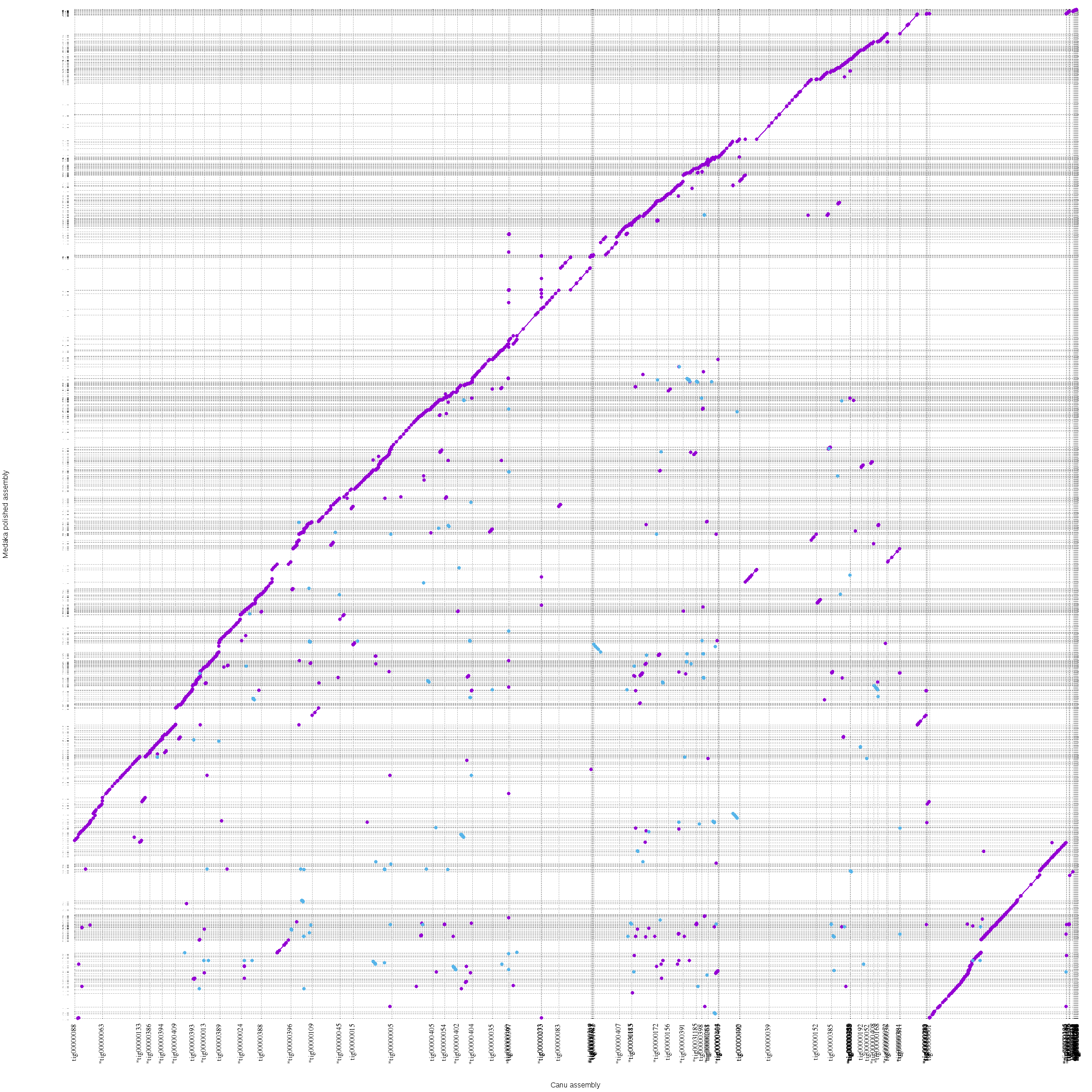
 8.2. When we try using different parameters to generate assembly, or we would like to compare your assembly to a reference, we can produce a dotplot between two assemblies. One way to produce this dotplot is to use Mummer package. The run_mummer.slurm script aligns the medaka polished Shasta assembly to the Canu assembly and creat a dotplot between the two assemblies.

cp /share/workshop/genome_assembly/jli/Nanopore/run.scripts/run_mummer.slurm .

sbatch -J nuc.${USER} run_mummer.sh

 When the job finishes, we should have a file named “canu.vs.shasta.png” in the “06-Mummer” directory. We can download it to our laptop for viewing. The assembly from Canu is on the X axis. The dotplot I generated is here.

 There is a very nice web service (Dgenies) that can produce a very nice plot. The source code can also be downloaded and compiled on your local machine. The result I got from running Dgenies is here

 8.3 The quality of an assembly may be assessed using Illumina whole genome sequencing data and kmer based methods. There are a few packages that can be used to carry out this step, such as KAT, yak, merqury, and quast. I will leave you on your own to explore this.

 8.4 One other potential way to assess the quality of an assembly is to use transcriptome data, such as IsoSeq or regular mRNASeq data.