
Make sure our workspace is setup properly and request resources on the cluster
mkdir -p /share/workshop/genome_assembly/$USER
cd /share/workshop/genome_assembly/$USER

srun -t 06:00:00 -c 24 -n 1 --mem 32000 --partition production --account genome_workshop --reservation genome_workshop --pty /bin/bash
aklog
Assessing Assembly Completeness
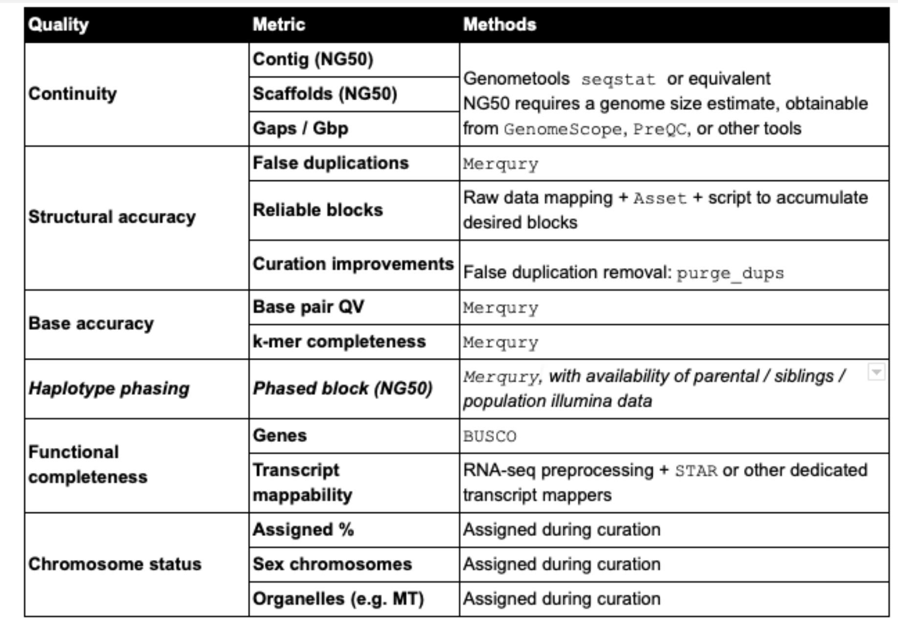
The VGP and EBP has published a set of Draft Assembly Statistics to aspire to.
They propose six broad quality categories (see table below)
- Continuity
- Structural accuracy
- Base accuracy
- Haplotype phasing
- Functional completeness
- Chromosome status
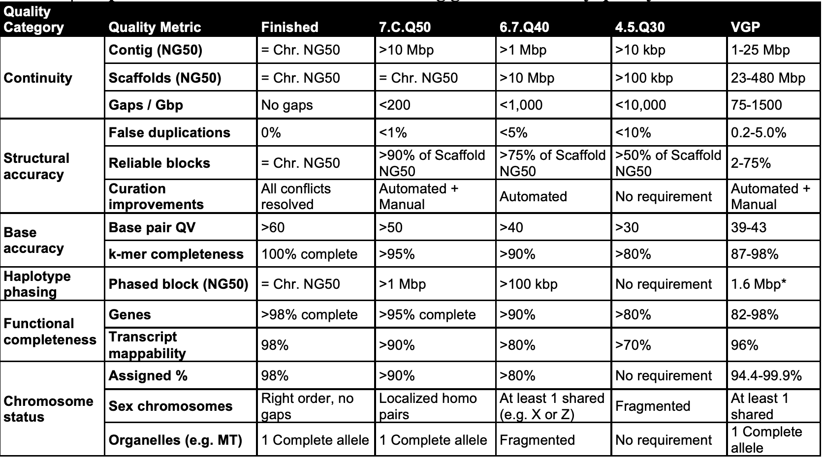
The 1st column are split into sub-metrics in the 2nd column. The recommendations for draft to finished qualities (columns 3–6) are based on those achieved in past studies, this study, and what we aspire to.
Quality of an assembly can be expressed in a 3 value notation, X.Y.Q = contig NG50 log10 value; scaffold NG50 log10 value; and QV value.
Assembly metrics
- N50
- N50 statistic defines assembly quality in terms of contiguity. Given a set of contigs, the N50 is defined as the sequence length of the shortest contig at 50% of the total genome length. N50 can be described as a weighted median statistic such that 50% of the entire assembly is contained in contigs or scaffolds equal to or larger than this value.
- L50
- Given a set of contigs, each with its own length, the L50 count is defined as the smallest number of contigs whose length sum makes up half of genome size.
- N90
- The N90 statistic is less than or equal to the N50 statistic; it is the length for which the collection of all contigs of that length or longer contains at least 90% of the sum of the lengths of all contigs.
- NG50
- Note that N50 is calculated in the context of the assembly size rather than the genome size. Therefore, comparisons of N50 values derived from assemblies of significantly different lengths are usually not informative, even if for the same genome. To address this, the authors of the Assemblathon competition came up with a new measure called NG50. The NG50 statistic is the same as N50 except that it is 50% of the known or estimated genome size that must be of the NG50 length or longer. This allows for meaningful comparisons between different assemblies.
Additional Requirements
Our experience has shown that currently, all (combinations of) automated processes generate assemblies with a variety of remaining errors, some of which are relatively easy to address and should be corrected before submission. We therefore propose that a set of quality control criteria are required to be met including:
-
separation of sequence of the target species from contaminants and other organisms such as symbionts/cobionts
-
explicit identification of a primary (haploid or pseudo-haploid) assembly, with additional sequence in a secondary bin that may contain either full alternate haplotypes or a set of haplotypic/other sequence from the individual
-
separation and explicit identification of organellar genomes
-
only A,C,G,T and N bases and removal of trailing Ns
We also encourage:
-
identification of discordances between raw data and resulting assembly to locate and remove structural errors (misjoins, missed joins and false duplications)
-
identification of sex chromosomes where possible
-
reconciliation with the known karyotype where it exists and this is possible.
Applications
Preforming some metrics
genometools seqstat
We can use genometools to get a number of assembly stats. In order to get NG50 values we need to provide it the estimate of the genome size determined by genomescope.
mkdir genometools
cd genometools
module load genometools/1.5.9
gt seqstat -contigs -genome 135000000 /share/workshop/genome_assembly/pacbio_2020_data_drosophila/hifi_long_read_diploid_ipa_assembly/RUN/14-final/final.p_ctg.fasta > diploid_ipa_assembly.stats
# number of contigs:     208
# genome length:         135000000
# total contigs length:  232197789
#    as % of genome:     172.00 %
# mean contig size:      1116335.52
# contig size first quartile: 78104
# median contig size:         148967
# contig size third quartile: 534433
# longest contig:             23464522
# shortest contig:            50222
# contigs > 500 nt:           208 (100.00 %)
# contigs > 1K nt:            208 (100.00 %)
# contigs > 10K nt:           208 (100.00 %)
# contigs > 100K nt:          135 (64.90 %)
# contigs > 1M nt:            37 (17.79 %)
# N50:                   7970785
# L50:                   9
# N80:                   1615167
# L80:                   29
# NG50:                  12556253
# LG50:                  4
# NG80:                  8941183
# LG80:                  8
Now lets take a look at the purged duplicates result.
gt seqstat -contigs -genome 135000000 /share/workshop/genome_assembly/pacbio_2020_data_drosophila/purge_dup_asm/final.purged.p_ctg.fasta > purged_ipa_assembly.stats
# number of contigs:     70
# genome length:         135000000
# total contigs length:  134186888
#    as % of genome:     99.40 %
# mean contig size:      1916955.54
# contig size first quartile: 105276
# median contig size:         314579
# contig size third quartile: 1030361
# longest contig:             23466353
# shortest contig:            50196
# contigs > 500 nt:           70 (100.00 %)
# contigs > 1K nt:            70 (100.00 %)
# contigs > 10K nt:           70 (100.00 %)
# contigs > 100K nt:          54 (77.14 %)
# contigs > 1M nt:            17 (24.29 %)
# N50:                   13488756
# L50:                   4
# N80:                   2484305
# L80:                   9
# NG50:                  13488756
# LG50:                  4
# NG80:                  2121280
# LG80:                  10
MERQURY
Merqury got alot of its inspiration from KAT K-mer Analysis Toolkit First we need some dependancies. Gonzalo Garcia from the Earlham Institute in the UK contributed to the last Genome Assembly workshop in 2018 discussing k-mers and KAT. Can see his materials here.
mkdir merqury_drosophila
cd merqury_drosophila/
ln -s /share/workshop/genome_assembly/pacbio_2020_data_drosophila/hifi_long_read_data/ELF_19kb.m64001_190914_015449.Q20.38X.fasta .
ln -s /share/workshop/genome_assembly/pacbio_2020_data_drosophila/purge_dup_asm/final.purged.*.fasta .

module load R
# Need argparse, ggplot2, scales
Rscript -e 'install.packages(c("argparse", "ggplot2", "scales"),repos = "http://cran.us.r-project.org")'

module load samtools
module load bedtools2
module load java/jdk11.0
module load igvtools

wget https://github.com/marbl/meryl/releases/download/v1.0/meryl-1.0.Linux-amd64.tar.xz
tar -xf meryl-1.0.Linux-amd64.tar.xz
export PATH=$PWD/meryl-1.0/Linux-amd64/bin:$PATH
Creating Meryl counts of the high quality PacBio HiFi data.
meryl count k=21 ELF_19kb.m64001_190914_015449.Q20.38X.fasta output pacbio.meryl
# This takes quite some time 30+ minutes
# Alternatively you can link mine
#ln -s /share/workshop/genome_assembly/msettles/merqury_drosophila/pacbio.meryl .
git clone https://github.com/marbl/merqury.git
export MERQURY=$PWD/merqury
ln -s $MERQURY/merqury.sh

less merqury.sh
./merqury.sh pacbio.meryl final.purged.p_ctg.fasta final.purged.a_ctg.fasta merqury_pacbio
# Took about an hour
spectra_cn and spectra_asm plots
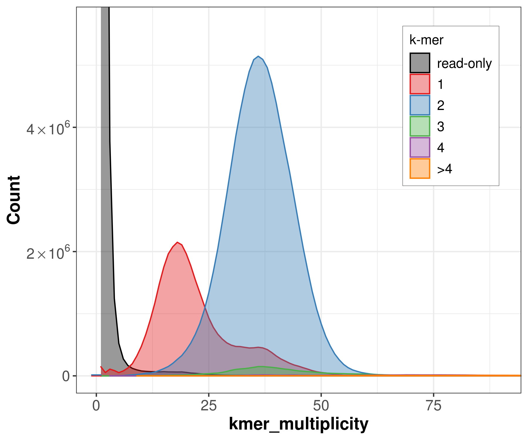
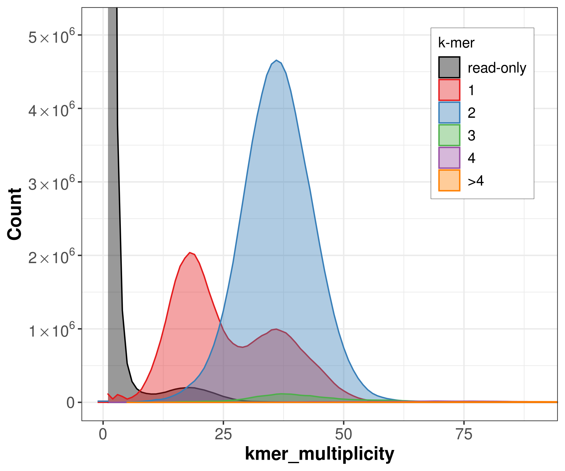
spectra_cn
We can count the canonical k-mers observed in the assembly and in the accurate, whole-genome read set (Here the original PacBio HiFi reads). A typical k-mer spectrum for a heterozygous diploid genome consists of two primary peaks, one representing k-mers that are 1-copy in the diploid genome (heterozygous, on a single haplotype) and one representing those that are 2-copy in the diploid genome (homozygous, on both haplotypes or two copies on one haplotype). The 2-copy k-mers appear with a frequency approximately equal to the average depth of sequencing coverage, where the 1-copy k-mers appear with frequency approximately equal to half the sequencing coverage. Using the multiplicity of the k-mer counts, and modeling the k-mer survival rate (i.e. how many k-mers are unaffected by sequencing error), it is possible to predict the size and repeat content of a genome from the k-mer spectrum alone.
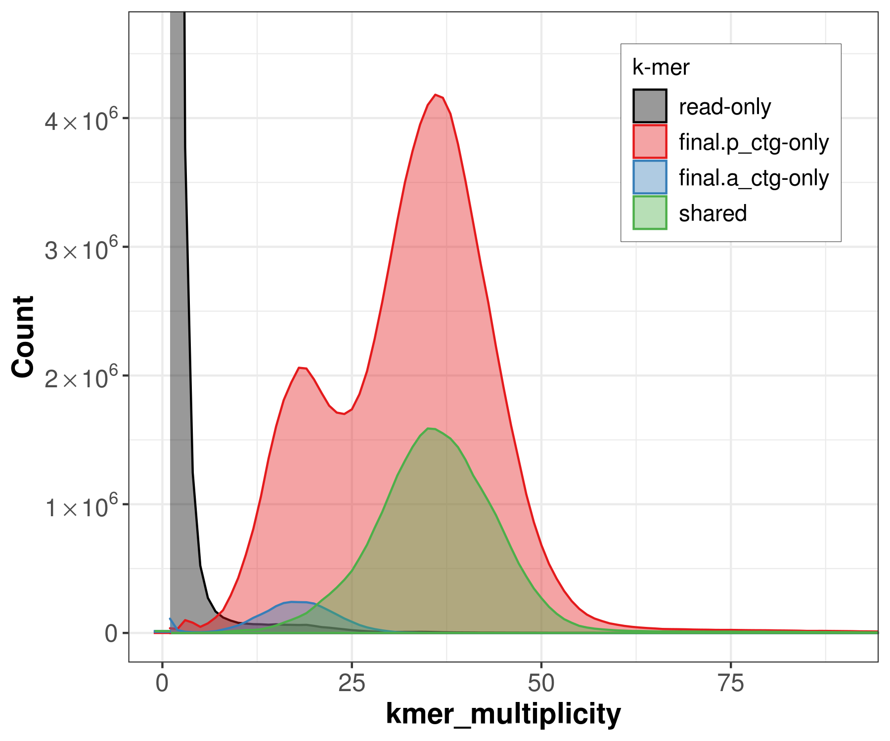
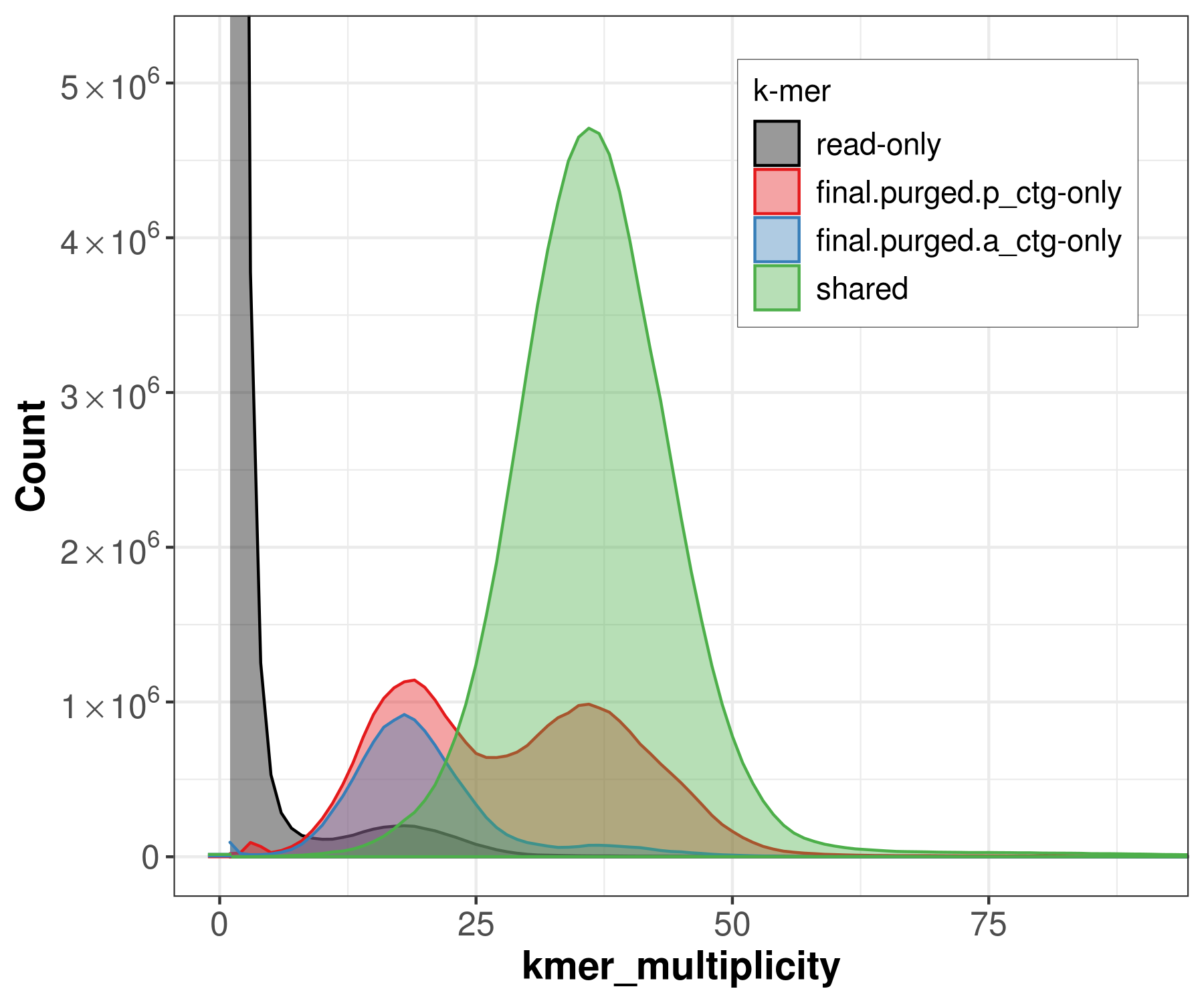
spectra_asm
Similar to the spectra-cn analysis, we can color each k-mer in the read set by the assembly in which it is found. This becomes useful when two haploid assemblies are evaluated. This way, we can detect k-mers that are present only in one assembly, k-mers shared in both assemblies, and k-mers not present in the assembly and only found in the read set.
file -> merqury_pacbio.spectra-cn.fl.png
file -> merqury_pacbio.spectra-asm.fl.png
QV values
We can also use k-mers to estimate the frequency of consensus errors in the assembly. We use a binomial model of k-mer survival, and assume all k-mers in the assembly should be found at least once in the read set. In brief, we estimate the probability P that a base in the assembly is correct.
file -> merqury_pacbio.qv
| Assembly | ASM_ONLY | TOTAL | QV | ERROR |
|---|---|---|---|---|
| final.purged.p_ctg | 4924 | 134184714 | 57.576 | 1.74744e-06 |
| final.purged.a_ctg | 10189 | 115249809 | 53.7571 | 4.21008e-06 |
| Both | 15113 | 249434523 | 55.3981 | 2.88528e-06 |
K-mer completeness
We define a “reliable k-mer” as a k-mer that is truly in the genome and unlikely to be caused by sequencing error. With exact k-mer counts, it is easy to filter out low-copy k-mers that are likely to represent sequencing errors. The k-mer completeness is calculated as the fraction of reliable k-mers in the read set that are also found in the assembly.
file -> completeness.stats
| Assembly | all | ASM | TOTAL | |
|---|---|---|---|---|
| final.purged.p_ctg | all | 116624064 | 131494201 | 88.6914 |
| final.purged.a_ctg | all | 97678031 | 131494201 | 74.2831 |
| both | all | 128428935 | 131494201 | 97.6689 |
Excercise
-
Given all the above what is the final X.Y.Q Assessment for this assembly.
-
Run the above excercise for each of the final resulting assemblies we’ve performed in this workshop, post the X.Y.Q Assessment in the Slack channel.