
Load libraries
library(Seurat)
library(biomaRt)
library(knitr)
library(kableExtra)
Load the Seurat object from part 1
load(file="original_seurat_object.RData")
experiment.aggregate
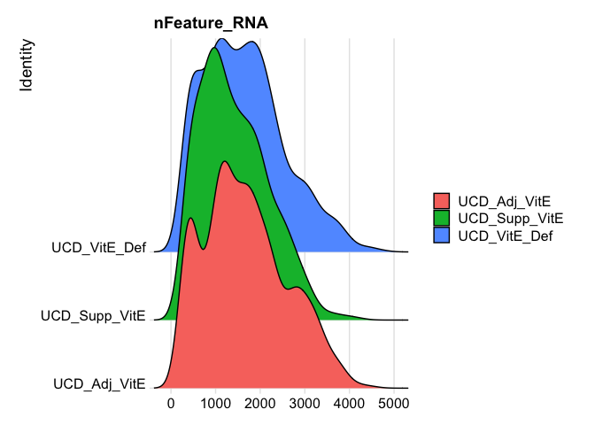
Some basic QA/QC of the metadata, print tables of the 5% quantiles.
Show 5% quantiles for number of genes per cell per sample
do.call("cbind", tapply(experiment.aggregate$nFeature_RNA, Idents(experiment.aggregate),quantile,probs=seq(0,1,0.05)))
RidgePlot(experiment.aggregate, features="nFeature_RNA")
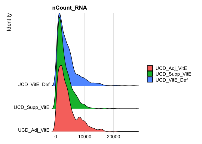
Show 5% quantiles for number of UMI per cell per sample
do.call("cbind", tapply(experiment.aggregate$nCount_RNA, Idents(experiment.aggregate),quantile,probs=seq(0,1,0.05)))
RidgePlot(experiment.aggregate, features="nCount_RNA")
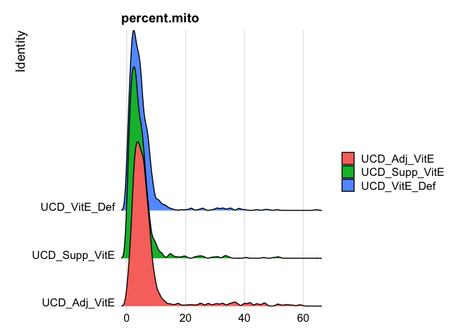
Show 5% quantiles for number of mitochondrial percentage per cell per sample
round(do.call("cbind", tapply(experiment.aggregate$percent.mito, Idents(experiment.aggregate),quantile,probs=seq(0,1,0.05))), digits = 3)
RidgePlot(experiment.aggregate, features="percent.mito")
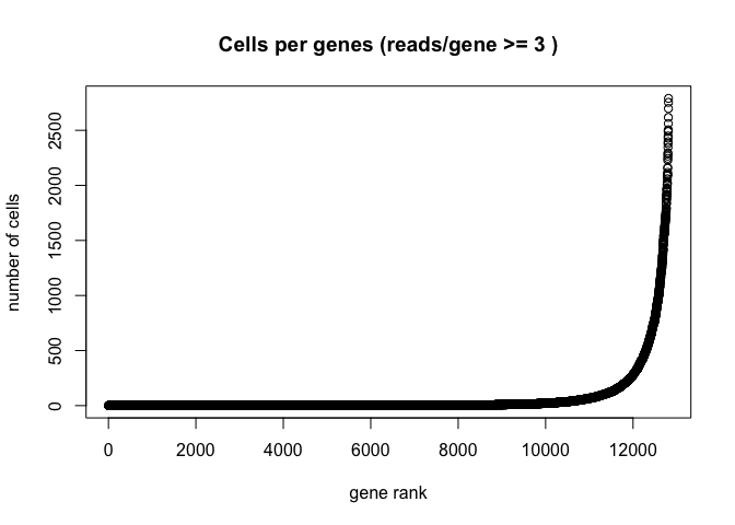
Plot the number of cells each gene is represented by
plot(sort(Matrix::rowSums(GetAssayData(experiment.aggregate) >= 3)) , xlab="gene rank", ylab="number of cells", main="Cells per genes (reads/gene >= 3 )")
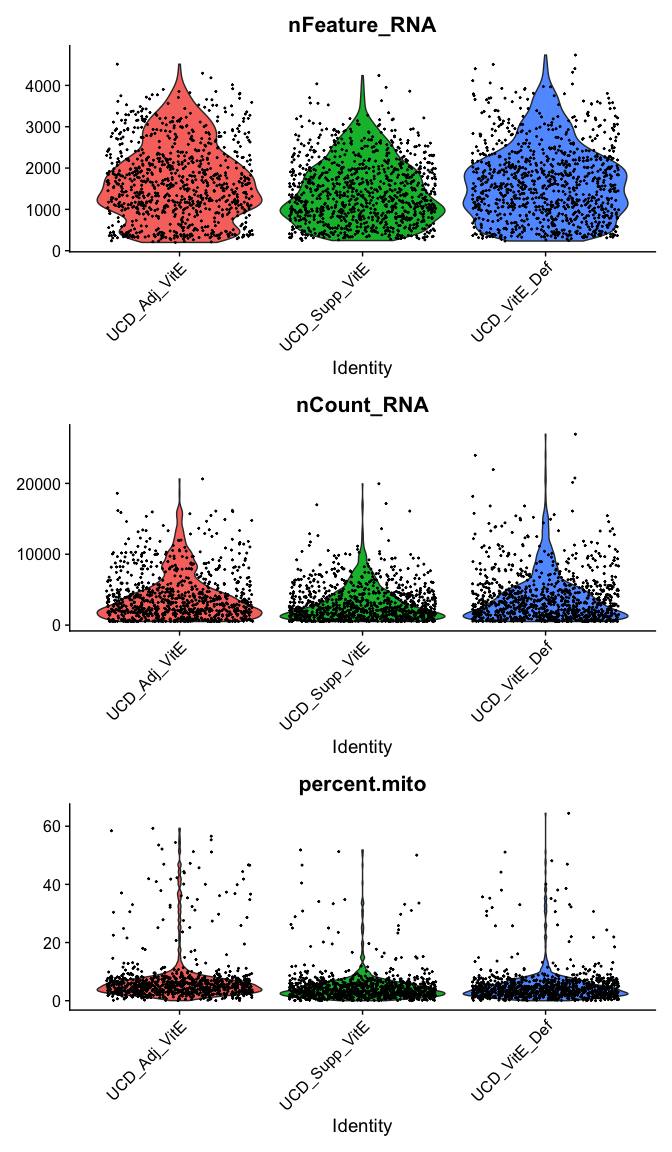
Violin plot of 1) number of genes, 2) number of UMI and 3) percent mitochondrial genes
VlnPlot(
  experiment.aggregate,
  features = c("nFeature_RNA", "nCount_RNA","percent.mito"),
  ncol = 1, pt.size = 0.3)
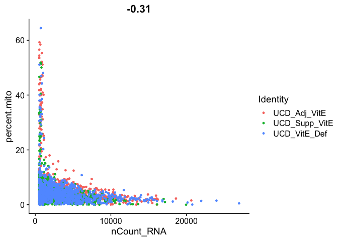
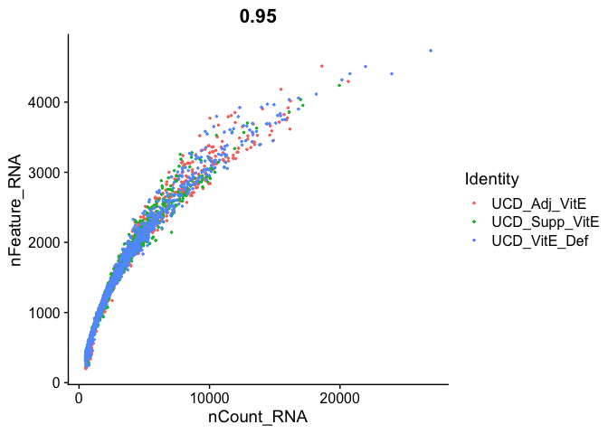
Gene Plot, scatter plot of gene expression across cells, (colored by sample)
FeatureScatter(experiment.aggregate, feature1 = "nCount_RNA", feature2 = "percent.mito")
FeatureScatter(
  experiment.aggregate, "nCount_RNA", "nFeature_RNA",
  pt.size = 0.5)
Cell filtering
We use the information above to filter out cells. Here we choose those that have percent mitochondrial genes max of 10% and unique UMI counts under 20,000 or greater than 500.
experiment.aggregate <- subset(experiment.aggregate, percent.mito <= 10)

experiment.aggregate <- subset(experiment.aggregate, nCount_RNA >= 500 & nCount_RNA <= 20000)

experiment.aggregate
You may also want to filter out additional genes.
When creating the base Seurat object we did filter out some genes, recall Keep all genes expressed in >= 10 cells. After filtering cells and you may want to be more aggressive with the gene filter. Seurat doesn’t supply such a function (that I can find), so below is a function that can do so, it filters genes requiring a min.value (log-normalized) in at least min.cells, here expression of 1 in at least 400 cells.
FilterGenes <-
 function (object, min.value=1, min.cells = 0, genes = NULL) {
   genes.use <- rownames(object)
   if (!is.null(genes)) {
     genes.use <- intersect(genes.use, genes)
     object@data <- GetAssayData(object)[genes.use, ]
   } else if (min.cells > 0) {
     num.cells <- Matrix::rowSums(GetAssayData(object) > min.value)
     genes.use <- names(num.cells[which(num.cells >= min.cells)])
     object = object[genes.use, ]
   }
  object <- LogSeuratCommand(object = object)
  return(object)
}

experiment.aggregate.genes <- FilterGenes(object = experiment.aggregate, min.value = 1, min.cells = 400)
experiment.aggregate.genes
table(Idents(experiment.aggregate))
Next we want to normalize the data
After filtering out cells from the dataset, the next step is to normalize the data. By default, we employ a global-scaling normalization method LogNormalize that normalizes the gene expression measurements for each cell by the total expression, multiplies this by a scale factor (10,000 by default), and then log-transforms the data.
?NormalizeData
experiment.aggregate <- NormalizeData(
  object = experiment.aggregate,
  normalization.method = "LogNormalize",
  scale.factor = 10000)
Calculate cell cycle using scran, add to meta data
(Scialdone A, Natarajana KN, Saraiva LR et al. (2015). Computational assignment of cell-cycle stage from single-cell transcriptome data. Methods 85:54–61])[https://pubmed.ncbi.nlm.nih.gov/26142758/]
Using the package scran, get the mouse cell cycle markers and a mapping of m There may be issues with timeout for the Biomart server, just keep trying
mm.pairs <- readRDS(system.file("exdata", "mouse_cycle_markers.rds", package="scran"))
# Convert to matrix for use in cycle
mat <- as.matrix(GetAssayData(experiment.aggregate))

# Convert rownames to ENSEMBL IDs, Using biomaRt
ensembl<- useMart(biomart = "ensembl", dataset = "mmusculus_gene_ensembl")

anno <- getBM( values=rownames(mat), attributes=c("mgi_symbol","ensembl_gene_id") , filters= "mgi_symbol"  ,mart=ensembl)

ord <- match(rownames(mat), anno$mgi_symbol) # use anno$mgi_symbol if via biomaRt
rownames(mat) <- anno$ensembl_gene_id[ord] # use anno$ensembl_gene_id if via biomaRt
drop <- which(is.na(rownames(mat)))
mat <- mat[-drop,]
cycles <- scran::cyclone(mat, pairs=mm.pairs)
tmp <- data.frame(cell.cycle = cycles$phases)
rownames(tmp) <- colnames(mat)
experiment.aggregate <- AddMetaData(experiment.aggregate, tmp)
Table of cell cycle (scran)
table(experiment.aggregate@meta.data$cell.cycle) %>% kable(caption = "Number of Cells in each Cell Cycle Stage", col.names = c("Stage", "Count"), align = "c") %>% kable_styling()
| Stage | Count |
|---|---|
| G1 | 2590 |
| G2M | 72 |
| S | 19 |
Calculate Cell-Cycle with Seurat, the list of genes comes with Seurat (only for human)
First need to convert to mouse symbols, we’ll use Biomart for that too.
table(Idents(experiment.aggregate))
convertHumanGeneList <- function(x){
  require("biomaRt")
  human = useMart("ensembl", dataset = "hsapiens_gene_ensembl")
  mouse = useMart("ensembl", dataset = "mmusculus_gene_ensembl")

  genes = getLDS(attributes = c("hgnc_symbol"), filters = "hgnc_symbol", values = x , mart = human, attributesL = c("mgi_symbol"), martL = mouse, uniqueRows=T)

  humanx <- unique(genes[, 2])

  # Print the first 6 genes found to the screen
  print(head(humanx))
  return(humanx)
}

m.s.genes <- convertHumanGeneList(cc.genes.updated.2019$s.genes)
m.g2m.genes <- convertHumanGeneList(cc.genes.updated.2019$g2m.genes)
# Create our Seurat object and complete the initialization steps
experiment.aggregate <- CellCycleScoring(experiment.aggregate, s.features = m.s.genes, g2m.features = m.g2m.genes, set.ident = TRUE)
Table of cell cycle (seurate)
table(experiment.aggregate@meta.data$Phase) %>% kable(caption = "Number of Cells in each Cell Cycle Stage", col.names = c("Stage", "Count"), align = "c") %>% kable_styling()
| Stage | Count |
|---|---|
| G1 | 945 |
| G2M | 854 |
| S | 882 |
Comparing the 2
table(scran=experiment.aggregate$cell.cycle, seurat=experiment.aggregate$Phase) %>% kable(caption = "Comparing scran to seurat cell cycle calls", align = "c") %>% kable_styling()
| G1 | G2M | S | |
|---|---|---|---|
| G1 | 914 | 817 | 859 |
| G2M | 26 | 31 | 15 |
| S | 5 | 6 | 8 |
Fixing the defualt “Ident” in Seurat
table(Idents(experiment.aggregate))
## So lets change it back to samplename
Idents(experiment.aggregate) <- "orig.ident"
table(Idents(experiment.aggregate))
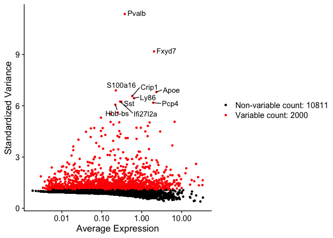
Identify variable genes
The function FindVariableFeatures identifies the most highly variable genes (default 2000 genes) by fitting a line to the relationship of log(variance) and log(mean) using loess smoothing, uses this information to standardize the data, then calculates the variance of the standardized data. This helps avoid selecting genes that only appear variable due to their expression level.
?FindVariableFeatures

experiment.aggregate <- FindVariableFeatures(
  object = experiment.aggregate,
  selection.method = "vst")

length(VariableFeatures(experiment.aggregate))
top10 <- head(VariableFeatures(experiment.aggregate), 10)

top10
vfp1 <- VariableFeaturePlot(experiment.aggregate)
vfp1 <- LabelPoints(plot = vfp1, points = top10, repel = TRUE)
vfp1
Question(s)
- Play some with the filtering parameters, see how results change?
- How do the results change if you use selection.method = “dispersion” or selection.method = “mean.var.plot”
Finally, lets save the filtered and normalized data
save(experiment.aggregate, file="pre_sample_corrected.RData")
Get the next Rmd file
download.file("https://raw.githubusercontent.com/ucdavis-bioinformatics-training/2020-Intro_Single_Cell_RNA_Seq/master/data_analysis/scRNA_Workshop-PART3.Rmd", "scRNA_Workshop-PART3.Rmd")
Session Information
sessionInfo()