Load libraries
library(Seurat)
library(ggplot2)
Load the Seurat object
load(file="pre_sample_corrected.RData")
experiment.aggregate
An object of class Seurat
12811 features across 2681 samples within 1 assay
Active assay: RNA (12811 features, 2000 variable features)
Now doing so for ‘real’
ScaleData - Scales and centers genes in the dataset. If variables are provided in vars.to.regress, they are individually regressed against each gene, and the resulting residuals are then scaled and centered unless otherwise specified. Here we regress out for sample (orig.ident) and percentage mitochondria (percent.mito).
?ScaleData
experiment.aggregate <- ScaleData(
  object = experiment.aggregate,
  vars.to.regress = c("cell.cycle", "percent.mito"))
Regressing out cell.cycle, percent.mito
Centering and scaling data matrix
Dimensionality reduction with PCA
Next we perform PCA (principal components analysis) on the scaled data.
?RunPCA
experiment.aggregate <- RunPCA(object = experiment.aggregate, features = VariableFeatures(object = experiment.aggregate))
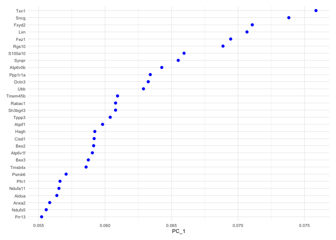
PC_ 1
Positive: Txn1, Sncg, Fxyd2, Lxn, Fez1, Rgs10, S100a10, Synpr, Atp6v0b, Ppp1r1a
Dctn3, Ubb, Tmem45b, Rabac1, Sh3bgrl3, Tppp3, Atpif1, Hagh, Cisd1, Bex2
Atp6v1f, Bex3, Tmsb4x, Psmb6, Pfn1, Ndufa11, Aldoa, Anxa2, Ndufs5, Prr13
Negative: Ptn, S100b, Mt1, Cbfb, Sv2b, Timp3, Ngfr, Nfia, Map2, Lynx1
Adcyap1, Gap43, Fxyd7, Enah, Thy1, Nefh, Scg2, Syt2, Nptn, Tmem229b
Igfbp7, Faim2, Kit, Zeb2, Nfib, Epb41l3, Cntnap2, Slc17a7, Ryr2, Ncdn
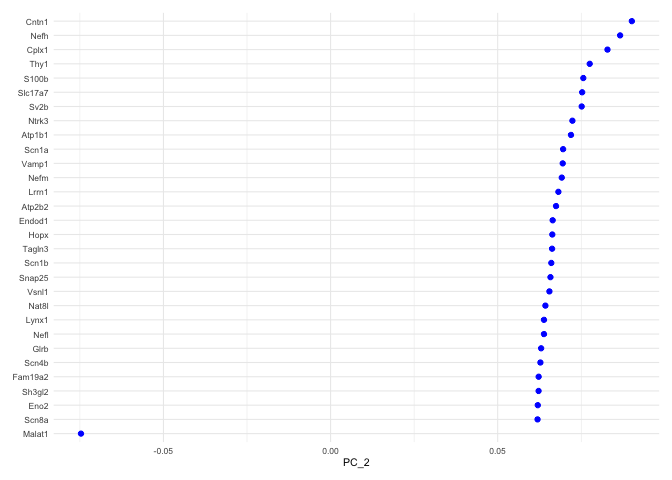
PC_ 2
Positive: Cntn1, Nefh, Cplx1, Thy1, S100b, Slc17a7, Sv2b, Ntrk3, Atp1b1, Scn1a
Vamp1, Nefm, Lrrn1, Atp2b2, Endod1, Hopx, Tagln3, Scn1b, Snap25, Vsnl1
Nat8l, Lynx1, Nefl, Glrb, Scn4b, Fam19a2, Sh3gl2, Eno2, Scn8a, Spock1
Negative: Malat1, Tmem233, Cd9, Cd24a, Prkca, Mal2, Dusp26, Carhsp1, Gna14, Crip2
Osmr, Cd44, Tmem158, Ift122, Id3, Gadd45g, Camk2a, Calca, Cd82, Hs6st2
Ctxn3, Emp3, Gm525, S100a6, Nppb, Socs2, Tac1, Sst, Arpc1b, Crip1
PC_ 3
Positive: P2ry1, Fam19a4, Gm7271, Rarres1, Th, Zfp521, Wfdc2, Tox3, Gfra2, Cdkn1a
D130079A08Rik, Rgs5, Kcnd3, Iqsec2, Pou4f2, Cd81, Cd34, Slc17a8, Rasgrp1, Casz1
Sorbs2, Id4, Dpp10, Piezo2, Zfhx3, Gm11549, Spink2, Gabra1, Igfbp7, Synpr
Negative: Calca, Basp1, Map1b, Ppp3ca, Gap43, Cystm1, Scg2, Tubb3, Calm1, Map7d2
Ncdn, Ift122, 6330403K07Rik, Epb41l3, Skp1a, Tmem233, Nmb, Dusp26, Tmem255a, Resp18
Crip2, Ntrk1, Tnfrsf21, Prkca, Fxyd7, Ywhag, Deptor, Camk2a, Mt3, Camk2g
PC_ 4
Positive: Adk, Etv1, Pvalb, Nsg1, Jak1, Tmem233, Tspan8, Nppb, Sst, Gm525
Htr1f, Slc17a7, Shox2, Spp1, Slit2, Nts, Cbln2, Osmr, Stxbp6, Cmtm8
Aldoc, Runx3, Cysltr2, Fam19a2, Klf5, Hapln4, Ptprk, Rasgrp2, Carhsp1, Nxph1
Negative: Gap43, Calca, Arhgdig, Stmn1, Tac1, 6330403K07Rik, Ngfr, Alcam, Kit, Ppp3ca
Smpd3, Fxyd6, Adcyap1, Atp1a1, Ntrk1, Tagln3, Gal, Tmem100, Gm7271, Chl1
Atp2b4, Mt3, Dclk1, Prune2, Tppp3, S100a11, Cnih2, Fbxo2, Fxyd7, Mgll
PC_ 5
Positive: Fxyd2, Rgs4, Acpp, Cpne3, Klf5, Zfhx3, Prune2, Nbl1, Cd24a, Gnb1
Phf24, Dgkz, Prkca, Parm1, Osmr, Ywhag, Tmem233, Jak1, Synpr, Kif5b
Tspan8, Plxnc1, Dpp10, Casz1, Ano3, Rasgrp1, P2ry1, Socs2, Nppb, Arpc1b
Negative: Mt1, Prdx1, Ptn, Dbi, B2m, Id3, Sparc, Mt2, Ifitm3, Ubb
Selenop, Mt3, Rgcc, Cryab, Timp3, Apoe, Uqcrb, Hspa1a, Phlda1, Tecr
Fxyd7, Dad1, Qk, Ier2, Fxyd1, Ifitm2, Selenom, Spcs1, Psmb2, Cebpd
Seurat then provides a number of ways to visualize the PCA results
Visualize PCA loadings
p <- VizDimLoadings(experiment.aggregate, dims = 1, ncol = 1)
p + theme_minimal(base_size = 8)
p <- VizDimLoadings(experiment.aggregate, dims = 2, ncol = 1)
p + theme_minimal(base_size = 8)
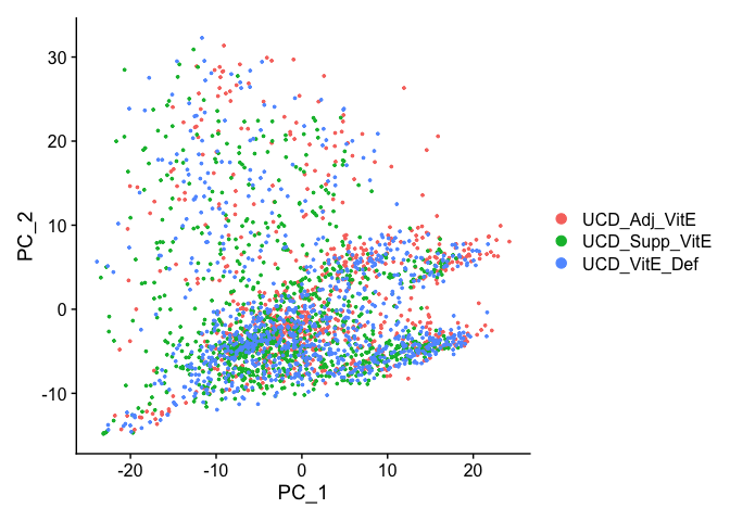
Principal components plot
DimPlot(
  object = experiment.aggregate, reduction = "pca")
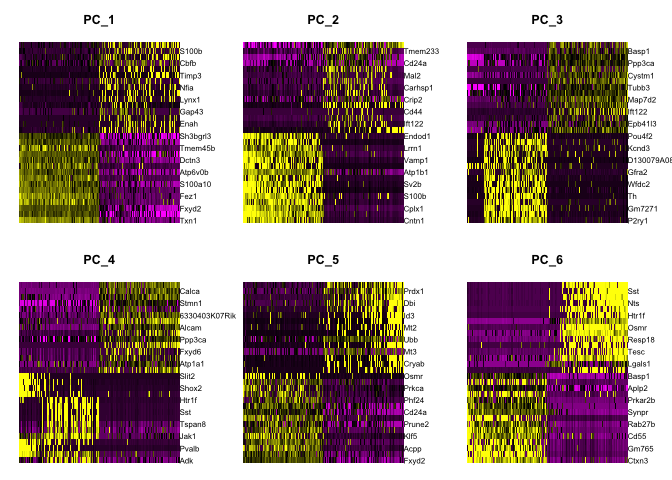
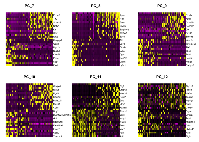
Draws a heatmap focusing on a principal component. Both cells and genes are sorted by their principal component scores. Allows for nice visualization of sources of heterogeneity in the dataset.
DimHeatmap(object = experiment.aggregate, dims = 1:6, cells = 500, balanced = TRUE)
DimHeatmap(object = experiment.aggregate, dims = 7:12, cells = 500, balanced = TRUE)
Selecting which PCs to use
To overcome the extensive technical noise in any single gene, Seurat clusters cells based on their PCA scores, with each PC essentially representing a metagene that combines information across a correlated gene set. Determining how many PCs to include downstream is therefore an important step.
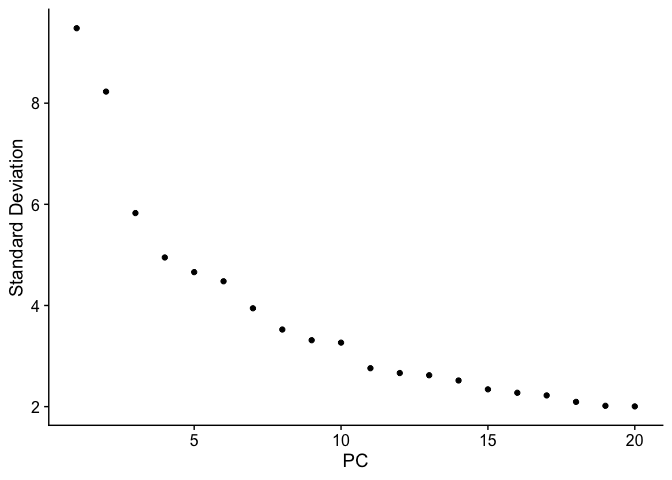
ElbowPlot plots the standard deviations (or approximate singular values if running PCAFast) of the principle components for easy identification of an elbow in the graph. This elbow often corresponds well with the significant PCs and is much faster to run. This is the traditional approach to selecting principal components.
ElbowPlot(experiment.aggregate)
The JackStraw function randomly permutes a subset of data, and calculates projected PCA scores for these ‘random’ genes, then compares the PCA scores for the ‘random’ genes with the observed PCA scores to determine statistical signifance. End result is a p-value for each gene’s association with each principal component. We identify significant PCs as those who have a strong enrichment of low p-value genes.
WARNING: TAKES A LONG TIME TO RUN
experiment.aggregate <- JackStraw(
    object = experiment.aggregate, dims = 40)
experiment.aggregate <- ScoreJackStraw(experiment.aggregate, dims = 1:40)
JackStrawPlot(object = experiment.aggregate, dims = 1:40)
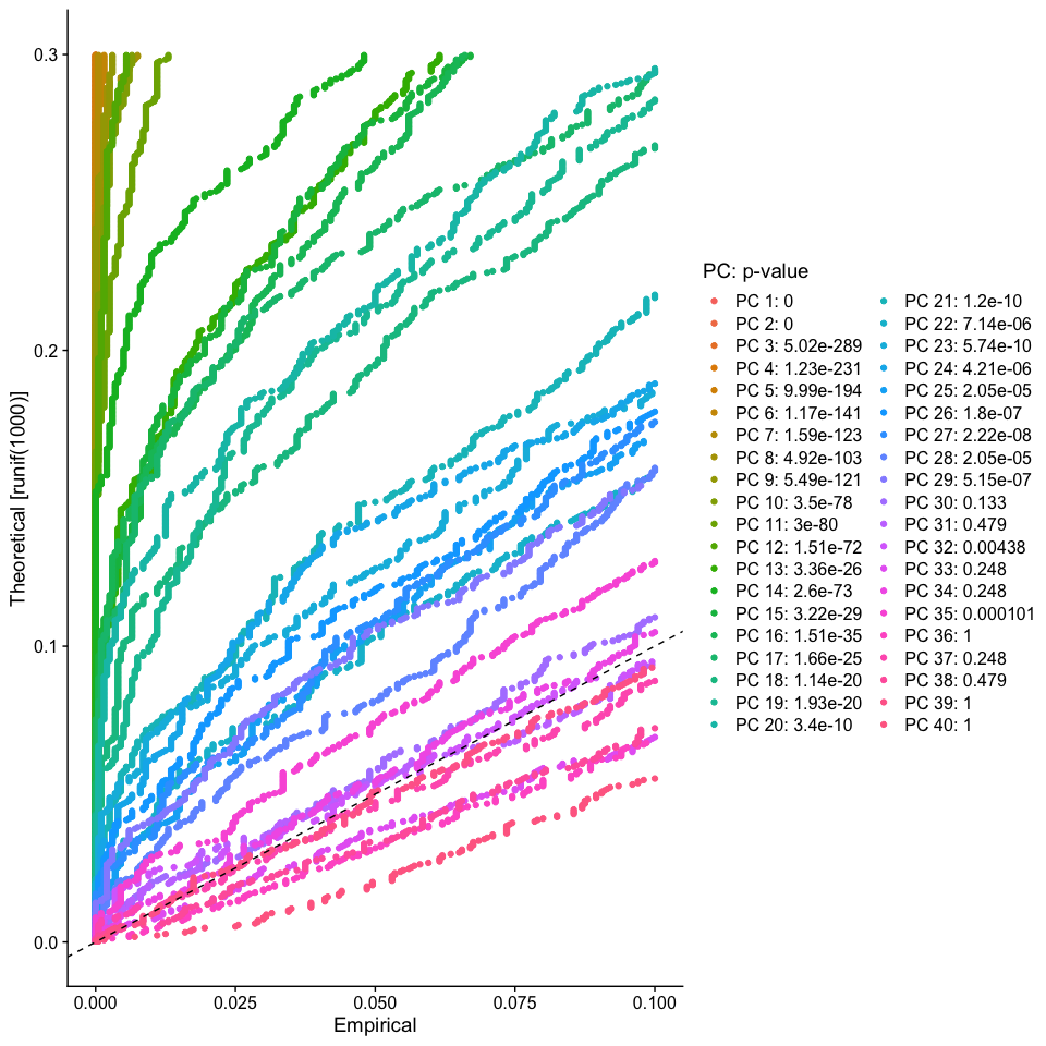
Looking at the results of the JackStraw plot, we determine to use the first 35 PCs
Finally, lets save the filtered and normalized data
save(experiment.aggregate, file="pca_sample_corrected.RData")
Get the next Rmd file
download.file("https://raw.githubusercontent.com/ucdavis-bioinformatics-training/2020-Intro_Single_Cell_RNA_Seq/master/data_analysis/scRNA_Workshop-PART5.Rmd", "scRNA_Workshop-PART5.Rmd")
R version 4.0.0 (2020-04-24)
Platform: x86_64-apple-darwin17.0 (64-bit)
Running under: macOS Catalina 10.15.4
Matrix products: default
BLAS: /Library/Frameworks/R.framework/Versions/4.0/Resources/lib/libRblas.dylib
LAPACK: /Library/Frameworks/R.framework/Versions/4.0/Resources/lib/libRlapack.dylib
locale:
[1] en_US.UTF-8/en_US.UTF-8/en_US.UTF-8/C/en_US.UTF-8/en_US.UTF-8
attached base packages:
[1] stats graphics grDevices datasets utils methods base
other attached packages:
[1] ggplot2_3.3.0 Seurat_3.1.5
loaded via a namespace (and not attached):
[1] httr_1.4.1 tidyr_1.0.3 jsonlite_1.6.1
[4] viridisLite_0.3.0 splines_4.0.0 leiden_0.3.3
[7] assertthat_0.2.1 BiocManager_1.30.10 renv_0.10.0
[10] yaml_2.2.1 ggrepel_0.8.2 globals_0.12.5
[13] pillar_1.4.4 lattice_0.20-41 glue_1.4.1
[16] reticulate_1.15 digest_0.6.25 RColorBrewer_1.1-2
[19] colorspace_1.4-1 cowplot_1.0.0 htmltools_0.4.0
[22] Matrix_1.2-18 plyr_1.8.6 pkgconfig_2.0.3
[25] tsne_0.1-3 listenv_0.8.0 purrr_0.3.4
[28] patchwork_1.0.0 scales_1.1.1 RANN_2.6.1
[31] Rtsne_0.15 tibble_3.0.1 farver_2.0.3
[34] ellipsis_0.3.1 withr_2.2.0 ROCR_1.0-11
[37] pbapply_1.4-2 lazyeval_0.2.2 survival_3.1-12
[40] magrittr_1.5 crayon_1.3.4 evaluate_0.14
[43] future_1.17.0 nlme_3.1-147 MASS_7.3-51.5
[46] ica_1.0-2 tools_4.0.0 fitdistrplus_1.1-1
[49] data.table_1.12.8 lifecycle_0.2.0 stringr_1.4.0
[52] plotly_4.9.2.1 munsell_0.5.0 cluster_2.1.0
[55] irlba_2.3.3 compiler_4.0.0 rsvd_1.0.3
[58] rlang_0.4.6 grid_4.0.0 ggridges_0.5.2
[61] RcppAnnoy_0.0.16 htmlwidgets_1.5.1 igraph_1.2.5
[64] labeling_0.3 rmarkdown_2.1 gtable_0.3.0
[67] codetools_0.2-16 reshape2_1.4.4 R6_2.4.1
[70] gridExtra_2.3 zoo_1.8-8 knitr_1.28
[73] dplyr_0.8.5 uwot_0.1.8 future.apply_1.5.0
[76] KernSmooth_2.23-16 ape_5.3 stringi_1.4.6
[79] parallel_4.0.0 Rcpp_1.0.4.6 vctrs_0.3.0
[82] sctransform_0.2.1 png_0.1-7 tidyselect_1.1.0
[85] xfun_0.13 lmtest_0.9-37
