Reminder of samples
- UCD_Adj_VitE
- UCD_Supp_VitE
- UCD_VitE_Def
Load libraries
library(Seurat)
library(ggplot2)
Load the Seurat object
load("clusters_seurat_object.RData")
experiment.merged
An object of class Seurat
12811 features across 2681 samples within 1 assay
Active assay: RNA (12811 features, 2000 variable features)
3 dimensional reductions calculated: pca, tsne, umap
Idents(experiment.merged) <- "RNA_snn_res.0.5"
#0. Setup
Load the final Seurat object, load libraries (also see additional required packages for each example)
#1. DE With Single Cell Data Using Limma
For differential expression using models more complex than those allowed by FindAllMarkers(), data from Seurat may be used in limma (https://www.bioconductor.org/packages/devel/bioc/vignettes/limma/inst/doc/usersguide.pdf)
We illustrate by comparing sample 1 to sample 2 within cluster 0:
library(limma)
cluster0 <- subset(experiment.merged, idents = '0')
expr <- as.matrix(GetAssayData(cluster0))

# Filter out genes that are 0 for every cell in this cluster
bad <- which(rowSums(expr) == 0)
expr <- expr[-bad,]

mm <- model.matrix(~0 + orig.ident, data = cluster0@meta.data)
fit <- lmFit(expr, mm)
head(coef(fit)) # means in each sample for each gene
orig.identUCD_Adj_VitE orig.identUCD_Supp_VitE orig.identUCD_VitE_Def
Xkr4 0.00000000 0.00000000 0.01244639
Sox17 0.00000000 0.01668876 0.00000000
Mrpl15 0.08176912 0.03552368 0.08691244
Lypla1 0.19102070 0.14361137 0.26607008
Tcea1 0.20114933 0.21041606 0.20030404
Rgs20 0.08977786 0.16701617 0.12833534
contr <- makeContrasts(orig.identUCD_Supp_VitE - orig.identUCD_Adj_VitE, levels = colnames(coef(fit)))
tmp <- contrasts.fit(fit, contrasts = contr)
tmp <- eBayes(tmp)
topTable(tmp, sort.by = "P", n = 20) # top 20 DE genes
logFC AveExpr t P.Value adj.P.Val B
Rpl21 -0.7556351 2.18376607 -5.855721 8.788450e-09 0.0001042925 9.539390
Rpl23a -0.6685951 2.20042706 -5.416089 9.625031e-08 0.0005711012 7.365993
Pcp4 -0.7945738 1.97307900 -5.080323 5.394231e-07 0.0021337779 5.806565
Rpl17 -0.6385737 2.03095291 -4.897874 1.324008e-06 0.0035478412 4.996517
Tmsb10 -0.5075879 3.39483016 -4.872780 1.494835e-06 0.0035478412 4.887183
Rpl24 -0.5884927 2.10921998 -4.770591 2.437077e-06 0.0048201321 4.447182
H3f3b -0.5739244 2.28377746 -4.559194 6.516427e-06 0.0098059796 3.563800
Rpl39 -0.5473089 2.24828560 -4.556050 6.610587e-06 0.0098059796 3.550936
Rps15 -0.5665492 1.98366043 -4.336666 1.762107e-05 0.0217259999 2.673438
Ndufa3 -0.4826286 0.75315056 -4.323873 1.863444e-05 0.0217259999 2.623495
Rps8 -0.5285119 2.56740433 -4.306059 2.013870e-05 0.0217259999 2.554177
Rpl32 -0.5363837 2.48366395 -4.272626 2.328052e-05 0.0230224951 2.424792
Zfp467 -0.2490624 0.16470870 -4.253390 2.529475e-05 0.0230902191 2.350772
Tshz2 -0.5320498 2.34028483 -4.148785 3.950113e-05 0.0318459666 1.953659
Tmsb4x -0.3725442 3.22438235 -4.144250 4.026341e-05 0.0318459666 1.936650
Alkal2 -0.1394787 0.05510728 -4.128964 4.293718e-05 0.0318459666 1.879445
Dbpht2 -0.4226453 0.63694021 -3.965965 8.417668e-05 0.0582822357 1.281665
Rps24 -0.5042936 1.54382120 -3.949370 9.003315e-05 0.0582822357 1.222063
Rpl10 -0.4695677 2.24688056 -3.940514 9.331444e-05 0.0582822357 1.190352
S100a10 -0.5110197 1.18692449 -3.917697 1.022983e-04 0.0606987101 1.108955
- logFC: log2 fold change (UCD_Supp_VitE/UCD_Adj_VitE)
- AveExpr: Average expression, in log2 counts per million, across all cells included in analysis (i.e. those in cluster 0)
- t: t-statistic, i.e. logFC divided by its standard error
- P.Value: Raw p-value from test that logFC differs from 0
- adj.P.Val: Benjamini-Hochberg false discovery rate adjusted p-value
The limma vignette linked above gives more detail on model specification.
2. Gene Ontology (GO) Enrichment of Genes Expressed in a Cluster
Loading required package: BiocGenerics
Loading required package: parallel
Attaching package: 'BiocGenerics'
The following objects are masked from 'package:parallel':
clusterApply, clusterApplyLB, clusterCall, clusterEvalQ, clusterExport, clusterMap, parApply, parCapply, parLapply, parLapplyLB, parRapply, parSapply, parSapplyLB
The following object is masked from 'package:limma':
plotMA
The following objects are masked from 'package:stats':
IQR, mad, sd, var, xtabs
The following objects are masked from 'package:base':
anyDuplicated, append, as.data.frame, basename, cbind, colnames, dirname, do.call, duplicated, eval, evalq, Filter, Find, get, grep, grepl, intersect, is.unsorted, lapply, Map, mapply, match, mget, order, paste, pmax, pmax.int, pmin, pmin.int, Position, rank, rbind, Reduce, rownames, sapply, setdiff, sort, table, tapply, union, unique, unsplit, which, which.max, which.min
Loading required package: graph
Loading required package: Biobase
Welcome to Bioconductor
Vignettes contain introductory material; view with 'browseVignettes()'. To cite Bioconductor, see 'citation("Biobase")', and for packages 'citation("pkgname")'.
Loading required package: GO.db
Loading required package: AnnotationDbi
Loading required package: stats4
Loading required package: IRanges
Loading required package: S4Vectors
Attaching package: 'S4Vectors'
The following object is masked from 'package:base':
expand.grid
Loading required package: SparseM
Attaching package: 'SparseM'
The following object is masked from 'package:base':
backsolve
groupGOTerms: GOBPTerm, GOMFTerm, GOCCTerm environments built.
Attaching package: 'topGO'
The following object is masked from 'package:IRanges':
members
# install org.Mm.eg.db from Bioconductor if not already installed (for mouse only)
cluster0 <- subset(experiment.merged, idents = '0')
expr <- as.matrix(GetAssayData(cluster0))
# Select genes that are expressed > 0 in at least 75% of cells (somewhat arbitrary definition)
n.gt.0 <- apply(expr, 1, function(x)length(which(x > 0)))
expressed.genes <- rownames(expr)[which(n.gt.0/ncol(expr) >= 0.75)]
all.genes <- rownames(expr)

# define geneList as 1 if gene is in expressed.genes, 0 otherwise
geneList <- ifelse(all.genes %in% expressed.genes, 1, 0)
names(geneList) <- all.genes

# Create topGOdata object
	GOdata <- new("topGOdata",
		ontology = "BP", # use biological process ontology
		allGenes = geneList,
		geneSelectionFun = function(x)(x == 1),
              annot = annFUN.org, mapping = "org.Mm.eg.db", ID = "symbol")
Building most specific GOs .....
Loading required package: org.Mm.eg.db
( 10610 GO terms found. )
Build GO DAG topology ..........
( 14634 GO terms and 34710 relations. )
Annotating nodes ...............
( 11709 genes annotated to the GO terms. )
# Test for enrichment using Fisher's Exact Test
	resultFisher <- runTest(GOdata, algorithm = "elim", statistic = "fisher")
-- Elim Algorithm --
the algorithm is scoring 2871 nontrivial nodes
parameters:
test statistic: fisher
cutOff: 0.01
Level 19: 1 nodes to be scored (0 eliminated genes)
Level 18: 1 nodes to be scored (0 eliminated genes)
Level 17: 1 nodes to be scored (0 eliminated genes)
Level 16: 6 nodes to be scored (0 eliminated genes)
Level 15: 16 nodes to be scored (0 eliminated genes)
Level 14: 32 nodes to be scored (24 eliminated genes)
Level 13: 72 nodes to be scored (31 eliminated genes)
Level 12: 108 nodes to be scored (429 eliminated genes)
Level 11: 178 nodes to be scored (762 eliminated genes)
Level 10: 255 nodes to be scored (790 eliminated genes)
Level 9: 324 nodes to be scored (1362 eliminated genes)
Level 8: 377 nodes to be scored (1501 eliminated genes)
Level 7: 453 nodes to be scored (1913 eliminated genes)
Level 6: 442 nodes to be scored (2135 eliminated genes)
Level 5: 323 nodes to be scored (2181 eliminated genes)
Level 4: 180 nodes to be scored (2184 eliminated genes)
Level 3: 83 nodes to be scored (2794 eliminated genes)
Level 2: 18 nodes to be scored (2794 eliminated genes)
Level 1: 1 nodes to be scored (2794 eliminated genes)
GenTable(GOdata, Fisher = resultFisher, topNodes = 20, numChar = 60)
GO.ID Term Annotated Significant Expected Fisher
1 GO:0002181 cytoplasmic translation 79 19 0.92 2.7e-20
2 GO:0006412 translation 518 50 6.06 3.5e-18
3 GO:0000028 ribosomal small subunit assembly 18 7 0.21 7.4e-10
4 GO:0000027 ribosomal large subunit assembly 29 7 0.34 3.2e-08
5 GO:0097214 positive regulation of lysosomal membrane permeability 2 2 0.02 0.00014
6 GO:0006880 intracellular sequestering of iron ion 2 2 0.02 0.00014
7 GO:0002227 innate immune response in mucosa 2 2 0.02 0.00014
8 GO:0000462 maturation of SSU-rRNA from tricistronic rRNA transcript (SS... 30 4 0.35 0.00039
9 GO:0061844 antimicrobial humoral immune response mediated by antimicrob... 14 3 0.16 0.00052
10 GO:0016198 axon choice point recognition 4 2 0.05 0.00080
11 GO:0071635 negative regulation of transforming growth factor beta produ... 5 2 0.06 0.00133
12 GO:0006605 protein targeting 230 9 2.69 0.00151
13 GO:0002679 respiratory burst involved in defense response 6 2 0.07 0.00198
14 GO:1902255 positive regulation of intrinsic apoptotic signaling pathway... 6 2 0.07 0.00198
15 GO:1905323 telomerase holoenzyme complex assembly 6 2 0.07 0.00198
16 GO:0007409 axonogenesis 357 13 4.18 0.00256
17 GO:1904667 negative regulation of ubiquitin protein ligase activity 7 2 0.08 0.00275
18 GO:0071637 regulation of monocyte chemotactic protein-1 production 7 2 0.08 0.00275
19 GO:0019731 antibacterial humoral response 7 2 0.08 0.00275
20 GO:0007612 learning 124 6 1.45 0.00332
- Annotated: number of genes (out of all.genes) that are annotated with that GO term
- Significant: number of genes that are annotated with that GO term and meet our criteria for “expressed”
- Expected: Under random chance, number of genes that would be expected to be annotated with that GO term and meeting our criteria for “expressed”
- Fisher: (Raw) p-value from Fisher’s Exact Test
#3. Weighted Gene Co-Expression Network Analysis (WGCNA)
WGCNA identifies groups of genes (“modules”) with correlated expression.
WARNING: TAKES A LONG TIME TO RUN
Loading required package: dynamicTreeCut
Loading required package: fastcluster
Attaching package: 'fastcluster'
The following object is masked from 'package:stats':
hclust
Attaching package: 'WGCNA'
The following object is masked from 'package:IRanges':
cor
The following object is masked from 'package:S4Vectors':
cor
The following object is masked from 'package:stats':
cor
options(stringsAsFactors = F)
datExpr <- t(as.matrix(GetAssayData(experiment.merged)))[,VariableFeatures(experiment.merged)]  # only use variable genes in analysis

net <- blockwiseModules(datExpr, power = 10,
  corType = "bicor", # use robust correlation
	networkType = "signed", minModuleSize = 10,
	reassignThreshold = 0, mergeCutHeight = 0.15,
	numericLabels = F, pamRespectsDendro = FALSE,
	saveTOMs = TRUE,
	saveTOMFileBase = "TOM",
	verbose = 3)
Calculating module eigengenes block-wise from all genes
Flagging genes and samples with too many missing values...
..step 1
..Working on block 1 .
TOM calculation: adjacency..
..will not use multithreading.
Fraction of slow calculations: 0.000000
..connectivity..
..matrix multiplication (system BLAS)..
..normalization..
..done.
..saving TOM for block 1 into file TOM-block.1.RData
....clustering..
....detecting modules..
....calculating module eigengenes..
....checking kME in modules..
..removing 67 genes from module 1 because their KME is too low.
..removing 43 genes from module 3 because their KME is too low.
..removing 2 genes from module 12 because their KME is too low.
..merging modules that are too close..
mergeCloseModules: Merging modules whose distance is less than 0.15
Calculating new MEs...
black blue brown green grey red turquoise yellow
11 80 21 12 1536 11 312 17
# Convert labels to colors for plotting
mergedColors = net$colors
# Plot the dendrogram and the module colors underneath
plotDendroAndColors(net$dendrograms[[1]], mergedColors[net$blockGenes[[1]]],
"Module colors",
dendroLabels = FALSE, hang = 0.03,
addGuide = TRUE, guideHang = 0.05)
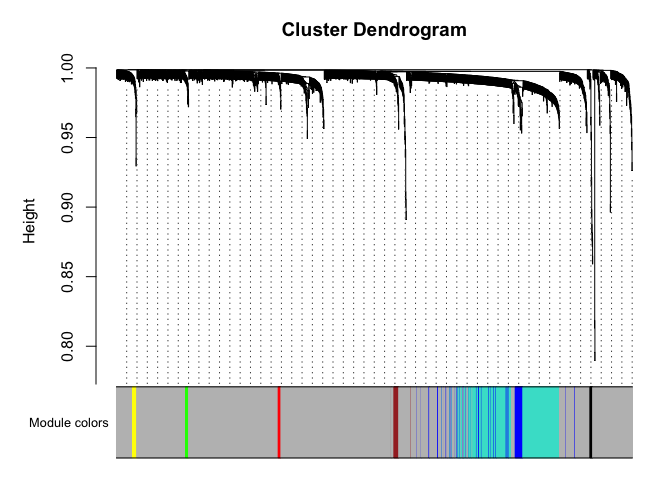 Genes in grey module are unclustered.
What genes are in the “blue” module?
colnames(datExpr)[net$colors == "blue"]
[1] "Lxn" "Txn1" "Grik1" "Fez1" "Tmem45b" "Synpr" "Tceal9" "Ppp1r1a" "Rgs10" "Nrn1" "Fxyd2" "Ostf1" "Lix1" "Sncb" "Paqr5" "Bex3" "Anxa5" "Gfra2" "Scg3" "Ppm1j" "Kcnab1" "Kcnip4" "Cadm1" "Isl2" "Pla2g7" "Tppp3" "Rgs4"
[28] "Tmsb4x" "Unc119" "Pmm1" "Ccdc68" "Rnf7" "Prr13" "Rsu1" "Pmp22" "Acpp" "Kcnip2" "Cdk15" "Mrps6" "Ebp" "Hexb" "Cdh11" "Dapk2" "Ano3" "Pde6d" "Snx7" "Dtnbp1" "Tubb2b" "Nr2c2ap" "Phf24" "Rcan2" "Fam241b" "Pmvk" "Slc25a4"
[55] "Zfhx3" "Dgkz" "Ndufv1" "Ptrh1" "1700037H04Rik" "Kif5b" "Sae1" "Sri" "Cpne3" "Dgcr6" "Cisd3" "Syt7" "Lhfpl3" "Dda1" "Ppp1ca" "Glrx3" "Stoml1" "Plagl1" "Lbh" "Degs1" "AI413582" "Car10" "Tlx2" "Parm1" "March11" "Cpe"
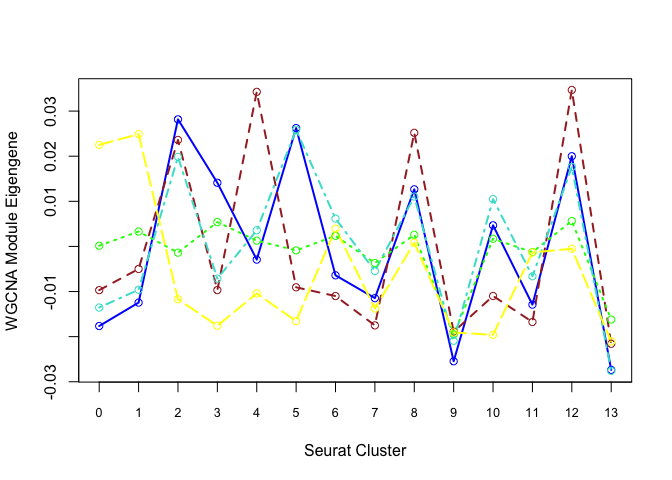
Each cluster is represented by a summary “eigengene”.
Plot eigengenes for each non-grey module by clusters from Seurat:
f <- function(module){
  eigengene <- unlist(net$MEs[paste0("ME", module)])
  means <- tapply(eigengene, Idents(experiment.merged), mean, na.rm = T)
  return(means)
}
modules <- c("blue", "brown", "green", "turquoise", "yellow")
plotdat <- sapply(modules, f)
matplot(plotdat, col = modules, type = "l", lwd = 2, xaxt = "n", xlab = "Seurat Cluster",
        ylab = "WGCNA Module Eigengene")
axis(1, at = 1:19, labels = 0:18, cex.axis = 0.8)
matpoints(plotdat, col = modules, pch = 21)
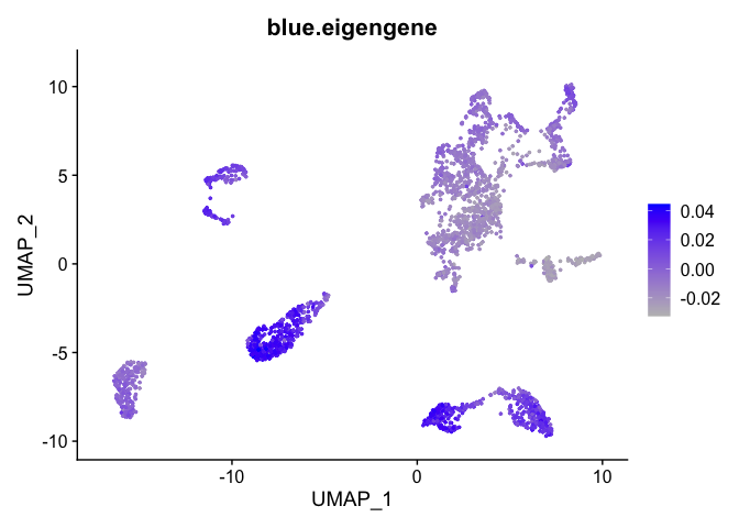
Can also plot the module onto the tsne plot
blue.eigengene <- unlist(net$MEs[paste0("ME", "blue")])
names(blue.eigengene) <- rownames(datExpr)
experiment.merged$blue.eigengene <- blue.eigengene
FeaturePlot(experiment.merged, features = "blue.eigengene", cols = c("grey", "blue"))
R version 4.0.0 (2020-04-24)
Platform: x86_64-apple-darwin17.0 (64-bit)
Running under: macOS Catalina 10.15.4
Matrix products: default
BLAS: /Library/Frameworks/R.framework/Versions/4.0/Resources/lib/libRblas.dylib
LAPACK: /Library/Frameworks/R.framework/Versions/4.0/Resources/lib/libRlapack.dylib
locale:
[1] en_US.UTF-8/en_US.UTF-8/en_US.UTF-8/C/en_US.UTF-8/en_US.UTF-8
attached base packages:
[1] stats4 parallel stats graphics grDevices datasets utils methods base
other attached packages:
[1] WGCNA_1.69 fastcluster_1.1.25 dynamicTreeCut_1.63-1 org.Mm.eg.db_3.11.1 topGO_2.40.0 SparseM_1.78 GO.db_3.11.1 AnnotationDbi_1.50.0 IRanges_2.22.1 S4Vectors_0.26.1 Biobase_2.48.0 graph_1.66.0 BiocGenerics_0.34.0 limma_3.44.1 ggplot2_3.3.0 Seurat_3.1.5
loaded via a namespace (and not attached):
[1] Rtsne_0.15 colorspace_1.4-1 ellipsis_0.3.1 ggridges_0.5.2 htmlTable_1.13.3 base64enc_0.1-3 rstudioapi_0.11 farver_2.0.3 leiden_0.3.3 listenv_0.8.0 ggrepel_0.8.2 bit64_0.9-7 codetools_0.2-16 splines_4.0.0 doParallel_1.0.15 impute_1.62.0 knitr_1.28 Formula_1.2-3 jsonlite_1.6.1 ica_1.0-2
[21] cluster_2.1.0 png_0.1-7 uwot_0.1.8 sctransform_0.2.1 BiocManager_1.30.10 compiler_4.0.0 httr_1.4.1 backports_1.1.7 assertthat_0.2.1 Matrix_1.2-18 lazyeval_0.2.2 acepack_1.4.1 htmltools_0.4.0 tools_4.0.0 rsvd_1.0.3 igraph_1.2.5 gtable_0.3.0 glue_1.4.1 RANN_2.6.1 reshape2_1.4.4
[41] dplyr_0.8.5 Rcpp_1.0.4.6 vctrs_0.3.0 preprocessCore_1.50.0 ape_5.3 nlme_3.1-147 iterators_1.0.12 lmtest_0.9-37 xfun_0.13 stringr_1.4.0 globals_0.12.5 lifecycle_0.2.0 irlba_2.3.3 renv_0.10.0 future_1.17.0 MASS_7.3-51.5 zoo_1.8-8 scales_1.1.1 RColorBrewer_1.1-2 yaml_2.2.1
[61] memoise_1.1.0 reticulate_1.15 pbapply_1.4-2 gridExtra_2.3 rpart_4.1-15 latticeExtra_0.6-29 stringi_1.4.6 RSQLite_2.2.0 foreach_1.5.0 checkmate_2.0.0 rlang_0.4.6 pkgconfig_2.0.3 matrixStats_0.56.0 evaluate_0.14 lattice_0.20-41 ROCR_1.0-11 purrr_0.3.4 labeling_0.3 patchwork_1.0.0 htmlwidgets_1.5.1
[81] cowplot_1.0.0 bit_1.1-15.2 tidyselect_1.1.0 RcppAnnoy_0.0.16 plyr_1.8.6 magrittr_1.5 R6_2.4.1 Hmisc_4.4-0 DBI_1.1.0 foreign_0.8-78 pillar_1.4.4 withr_2.2.0 fitdistrplus_1.1-1 nnet_7.3-13 survival_3.1-12 tibble_3.0.1 future.apply_1.5.0 tsne_0.1-3 crayon_1.3.4 KernSmooth_2.23-16
[101] plotly_4.9.2.1 rmarkdown_2.1 jpeg_0.1-8.1 grid_4.0.0 data.table_1.12.8 blob_1.2.1 digest_0.6.25 tidyr_1.0.3 munsell_0.5.0 viridisLite_0.3.0
