
For a non-Rmd version of this code, download the Velocyto.R script.
Project set-up
We begin by loading required packages.
library(Seurat)
library(ggplot2)
library(velocyto.R)
library(SeuratWrappers)
And storing the location and names of the input data.
data_location <- "data_download/"
samples <- c("sample1", "sample2", "sample3")
I prefer to use a few custom colorblind-friendly palettes, so we will set those up now. The palettes used in this exercise were developed by Paul Tol. You can learn more about them on Tol’s webpage.
tol_high_contrast_palette <- c("#DDAA33", "#BB5566", "#004488")
tol_vibrant_palette <- c("#0077BB", "#33BBEE", "#009988",
                         "#EE7733", "#CC3311", "#EE3377",
                         "#BBBBBB")
tol_muted_palette <- c("#332288", "#88CCEE", "#44AA99",
                       "#117733", "#999933", "#DDCC77",
                       "#CC6677", "#882255", "#AA4499")
Seurat
For completeness, and to practice integrating existing analyses with our velocyto analysis, we will run the cellranger count output through a basic Seurat analysis, creating a separate Seurat object, before we load in the loom files and begin our velocity analysis. For greater detail on single cell RNA-Seq analysis, see the course materials here.
The material in this section is not required to run the velocity analysis. We will be integrating this standard single cell RNA-Seq experiment with our velocity analysis in the third section. If you are in a hurry, you can skip this section. If you do so, you will need to make a few changes to the code in the Velocyto section, and, of course, you will not be able to execute the section on integrating the two analyses.
raw10x <- lapply(samples, function(i){
  d10x <- Read10X_h5(file.path(data_location, paste0(i, "_raw_feature_bc_matrix.h5")))
  colnames(d10x$`Gene Expression`) <- paste(sapply(strsplit(colnames(d10x$`Gene Expression`),split="-"),'[[',1L),i,sep="-")
  colnames(d10x$`Antibody Capture`) <- paste(sapply(strsplit(colnames(d10x$`Antibody Capture`),split="-"),'[[',1L),i,sep="-")
  d10x
})
names(raw10x) <- samples
gex <- CreateSeuratObject(do.call("cbind", lapply(raw10x,"[[", "Gene Expression")),
project = "cellranger multi",
min.cells = 0,
min.features = 300,
names.field = 2,
names.delim = "\\-")
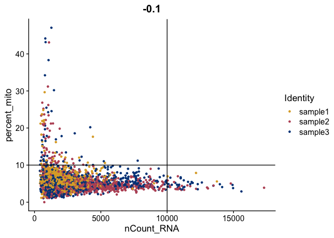
gex$percent_mito <- PercentageFeatureSet(gex, pattern = "^MT-")
FeatureScatter(gex,
feature1 = "nCount_RNA",
feature2 = "percent_mito",
shuffle = TRUE) +
geom_vline(xintercept = 10000) +
geom_hline(yintercept = 10) +
scale_color_manual(values = tol_high_contrast_palette)
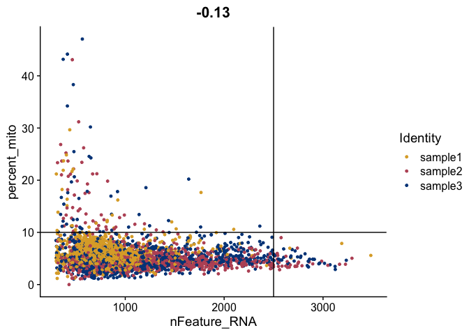
FeatureScatter(gex,
               feature1 = "nFeature_RNA",
               feature2 = "percent_mito",
               shuffle = TRUE) +
  geom_vline(xintercept = 2500) +
  geom_hline(yintercept = 10) +
  scale_color_manual(values = tol_high_contrast_palette)
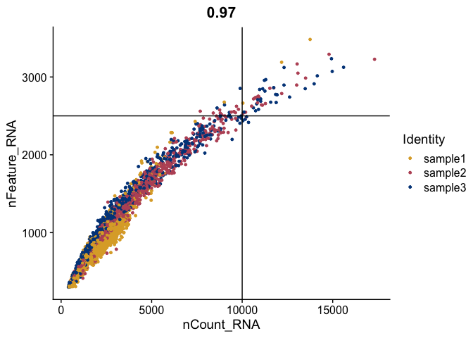
FeatureScatter(gex,
               feature1 = "nCount_RNA",
               feature2 = "nFeature_RNA",
               shuffle = TRUE) +
  geom_vline(xintercept = 10000) +
  geom_hline(yintercept = 2500) +
  scale_color_manual(values = tol_high_contrast_palette)
gex <- subset(gex, percent_mito <= 10)
gex <- subset(gex, nCount_RNA <= 10000)
gex <- subset(gex, nFeature_RNA >= 500)
table(gex$orig.ident)
gex <- NormalizeData(object = gex,
                     normalization.method = "LogNormalize",
                     scale.factor = 10000)

gex <- CellCycleScoring(object = gex,
                        s.features = cc.genes$s.genes,
                        g2m.features = cc.genes$g2m.genes,
                        set.ident = FALSE)
gex <- ScaleData(object = gex,
                 vars.to.regress = c("S.Score",
                                     "G2M.Score",
                                     "percent_mito",
                                     "nFeature_RNA"))
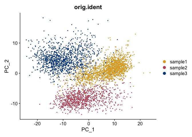
gex <- RunPCA(object = gex,
              npcs = 100,
              features = rownames(gex),
              verbose = FALSE)
DimPlot(object = gex,
        reduction = "pca",
        group.by = "orig.ident",
        shuffle = TRUE) +
  scale_color_manual(values = tol_high_contrast_palette)
gex <- FindNeighbors(object = gex,
                     reduction = "pca",
                     dims = c(1:50),
                     verbose = FALSE)
gex <- FindClusters(object = gex,
                    resolution = seq(0.25, 2, 0.25),
                    verbose = FALSE)
sapply(grep("res", colnames(gex@meta.data), value = TRUE),
       function(x) {length(unique(gex@meta.data[,x]))})
gex <- RunUMAP(object = gex,
               reduction = "pca",
               dims = c(1:50),
               verbose = FALSE)
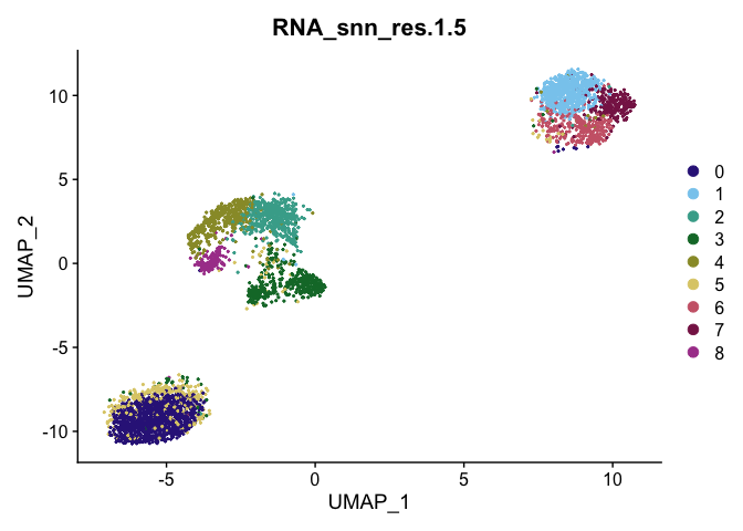
DimPlot(object = gex,
        reduction = "umap",
        group.by = "RNA_snn_res.1.5",
        shuffle = TRUE) +
  scale_color_manual(values = tol_muted_palette)
Velocyto
The velocyto workflow consists of a command line tool for data reduction, which generates counts tables for spliced and unspliced transcripts, and an R package, which calculates RNA velocity. The method is described in La Manno et al., 2018. This exercise uses the output from velocity data reduction.
Read in loom files
The velocyto input files are loom files, a specialized HDF5 file type designed to store large matrices (e.g. counts tables) and accompanying metadata. Each loom file contains three counts tables for a single sample: spliced transcripts, unspliced transcripts, and ambiguous transcripts.
Let’s load the spliced and unspliced counts tables into a Seurat object, renaming the columns to match the cell names generated by cellranger count.
reformatLoomColnames <- function(loomObject, assay, id){
  paste(substr(colnames(loomObject[[assay]]), 25, 40), id, sep = "-")
}

loom_data <- lapply(samples, function(sample_id){
  loom_object <- ReadVelocity(file.path(data_location,
                                        paste0(sample_id, ".loom")))
  colnames(loom_object$spliced) <- reformatLoomColnames(
    loomObject = loom_object,
    assay = "spliced",
    id = sample_id)
  colnames(loom_object$unspliced) <- reformatLoomColnames(
    loomObject = loom_object,
    assay = "unspliced",
    id = sample_id)
  colnames(loom_object$ambiguous) <- reformatLoomColnames(
    loomObject = loom_object,
    assay = "ambiguous",
    id = sample_id)
  loom_object
})
names(loom_data) <- samples

loom_aggregate <- lapply(c("spliced", "unspliced"), function(assay){
  do.call("cbind", lapply(loom_data,"[[", assay))
})
names(loom_aggregate) <- c("spliced", "unspliced")
vel <- CreateSeuratObject(counts = loom_aggregate$spliced,
                          project = "Advanced Topics Workshop",
                          assay = "spliced",
                          min.cells = 0,
                          min.features = 0,
                          names.field = 2,
                          names.delim = "\\-")
vel[["unspliced"]] <- CreateAssayObject(counts = loom_aggregate$unspliced)
Select cells used in gene expression analysis
The set of cells (columns) generated by the velocyto command line tool is not identical to the set of cells generated by cellranger count. How much do they differ? If you did not run the code in the initial Seurat section above, you will not be able to make this comparison.
gex
vel
length(which(is.element(colnames(vel), colnames(gex))))
Let’s subset our data to match our initial Seurat analysis. If you did not run the initial Seurat section, change the code to subset your cells in some other way, or simply use all cells.
vel <- vel[rownames(gex), colnames(gex)]
Run Seurat
In addition to the counts tables, velocyto requires the Seurat object’s nearest neighbor graph and reductions slot. Let’s first calculate these from our velocyto data.
vel <- NormalizeData(vel, verbose = FALSE)
vel <- ScaleData(vel, verbose = FALSE)
vel <- RunPCA(vel, features = rownames(vel), verbose = FALSE)
vel_reduction <- FindNeighbors(vel, dims = 1:50, verbose = FALSE)
vel_reduction <- FindClusters(vel_reduction, verbose = FALSE)
vel_reduction <- RunUMAP(vel_reduction, dims = 1:50, verbose = FALSE)
Alternatively, we can import the nearest neighbor graph, cluster assignments, and reduction embeddings from our initial Seurat analysis.
vel_integrated <- vel
# nearest neighbor graph
vel_integrated@graphs[["RNA_nn"]] <- gex@graphs[["RNA_nn"]][colnames(vel),
                                                            colnames(vel)]
# cluster assignments
vel_integrated <- AddMetaData(object = vel_integrated,
                              metadata = FetchData(gex,
                                                   vars = "RNA_snn_res.1.5",
                                                   cells = colnames(vel)),
                              col.name = "gex.clusters")
# UMAP
vel_integrated@reductions[["umap"]] <- CreateDimReducObject(embeddings = as.matrix(FetchData(gex, vars = c("UMAP_1", "UMAP_2"), cells = colnames(vel))), assay = "RNA")
Run velocity analysis
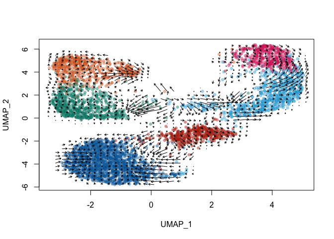
Finally we can run the velocity analysis! Let’s do the version that uses the velocity data for the nearest neighbor graph and UMAP embeddings first.
vel_reduction <- RunVelocity(vel_reduction,
                             deltaT = 1,
                             kCells = 25,
                             fit.quantile = 0.02,
                             verbose = FALSE)

ident_colors <- tol_vibrant_palette
names(ident_colors) <- levels(vel_reduction)
cell_colors <- ident_colors[Idents(vel_reduction)]
names(cell_colors) <- colnames(vel_reduction)
show.velocity.on.embedding.cor(emb = Embeddings(vel_reduction,
                                                reduction = "umap"),
                               vel = Tool(vel_reduction,
                                          slot = "RunVelocity"),
                               n = 200,
                               scale = "sqrt",
                               xlab = colnames(Embeddings(vel_reduction,
                                                          reduction = "umap"))[1],
                               ylab = colnames(Embeddings(vel_reduction,
                                                          reduction = "umap"))[2],
                               cell.colors = ac(x = cell_colors, alpha = 0.5),
                               cex = 0.8,
                               arrow.scale = 3,
                               show.grid.flow = TRUE,
                               min.grid.cell.mass = 0.5,
                               grid.n = 40,
                               arrow.lwd = 1,
                               do.par = FALSE,
                               cell.border.alpha = 0.1)
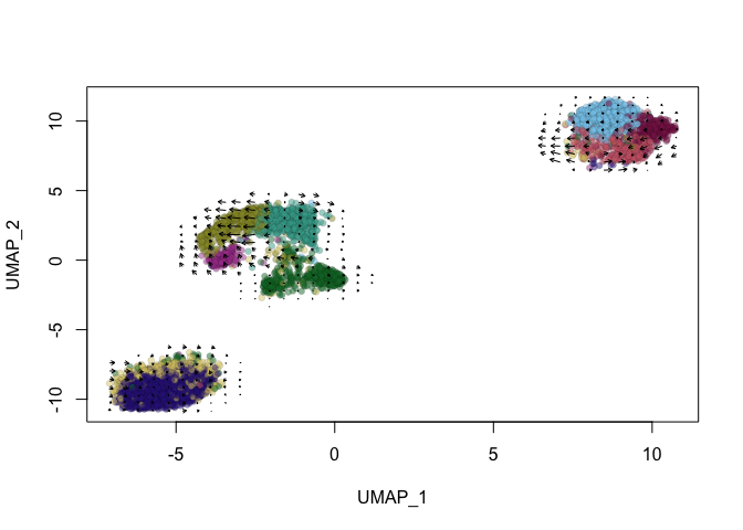
Next, let’s use the nearest neighbor graph and UMAP embeddings imported from the inital Seurat analysis.
vel_integrated <- RunVelocity(vel_integrated,
                             deltaT = 1,
                             kCells = 25,
                             fit.quantile = 0.02,
                             verbose = FALSE)
ident_colors <- tol_muted_palette
names(ident_colors) <- levels(vel_integrated$gex.clusters)
cell_colors <- ident_colors[vel_integrated$gex.clusters]
names(cell_colors) <- colnames(vel_integrated)
show.velocity.on.embedding.cor(emb = Embeddings(vel_integrated,
                                                reduction = "umap"),
                               vel = Tool(vel_integrated,
                                          slot = "RunVelocity"),
                               n = 200,
                               scale = "sqrt",
                               xlab = colnames(Embeddings(vel_integrated,
                                                          reduction = "umap"))[1],
                               ylab = colnames(Embeddings(vel_integrated,
                                                          reduction = "umap"))[2],
                               cell.colors = ac(x = cell_colors, alpha = 0.5),
                               cex = 0.8,
                               arrow.scale = 3,
                               show.grid.flow = TRUE,
                               min.grid.cell.mass = 0.5,
                               grid.n = 40,
                               arrow.lwd = 1,
                               do.par = FALSE,
                               cell.border.alpha = 0.1)
Session Information
sessionInfo()