Home
Introduction and Lectures
Intro to the Workshop and Core
Support
Using Slack in this workshop
Using Zoom in this workshop
Cheat Sheets
Software and Links
Scripts
Prerequisites
CLI
R
More Materials - Intro CLI
More Materials - Intro R
Velocity Analysis
Velocity data reduction
Prepare for Velocity analysis
Velocity data analysis
Monocle Trajectory Analysis
Prepare for Monocle
Monocle
ETC
Closing thoughts
Github page
Biocore website

Trajectory Analysis with Monocle 3

Monocle, from the Trapnell Lab, is a piece of the TopHat suite (for RNAseq) that performs among other things differential expression, trajectory, and pseudotime analyses on single cell RNA-Seq data. A very comprehensive tutorial can be found on the Trapnell lab website. We will be using Monocle3, which is still in the “beta” phase of its development and hasn’t been updated in a few years. The development branch however has some activity in the last year in preparation for Monocle3.1.

library(monocle3)
library(Seurat)
library(SeuratWrappers)
library(patchwork)
#library(dplyr)

set.seed(1234)

I prefer to use a few custom colorblind-friendly palettes, so we will set those up now. The palettes used in this exercise were developed by Paul Tol. You can learn more about them on Tol’s webpage.

tol_high_contrast_palette <- c("#DDAA33", "#BB5566", "#004488")
tol_vibrant_palette <- c("#0077BB", "#33BBEE", "#009988",
                         "#EE7733", "#CC3311", "#EE3377",
                         "#BBBBBB")
tol_muted_palette <- c("#332288", "#88CCEE", "#44AA99",
                       "#117733", "#999933", "#DDCC77",
                       "#CC6677", "#882255", "#AA4499")

Project set-up

Because Seurat is now the most widely used package for single cell data analysis we will want to use Monocle with Seurat. For greater detail on single cell RNA-Seq analysis, see the Introductory course materials here.

Loading data into Seurat

data_location <- "data_download/"
samples <- c("sample1", "sample2", "sample3")

raw10x <- lapply(samples, function(i){
  d10x <- Read10X_h5(file.path(data_location, paste0(i, "_raw_feature_bc_matrix.h5")))
  colnames(d10x$`Gene Expression`) <- paste(sapply(strsplit(colnames(d10x$`Gene Expression`),split="-"),'[[',1L),i,sep="-")
  colnames(d10x$`Antibody Capture`) <- paste(sapply(strsplit(colnames(d10x$`Antibody Capture`),split="-"),'[[',1L),i,sep="-")
  d10x
})

Genome matrix has multiple modalities, returning a list of matrices for this genome Genome matrix has multiple modalities, returning a list of matrices for this genome Genome matrix has multiple modalities, returning a list of matrices for this genome

names(raw10x) <- samples
trA <- CreateSeuratObject(do.call("cbind", lapply(raw10x,"[[", "Gene Expression")),
                          project = "cellranger multi",
                          min.cells = 0,
                          min.features = 300,
                          names.field = 2,
                          names.delim = "\\-")
trA$percent_mito <- PercentageFeatureSet(trA, pattern = "^MT-")

trA <- subset(trA, percent_mito <= 10)
trA <- subset(trA, nCount_RNA <= 10000)
trA <- subset(trA, nFeature_RNA >= 500)
table(trA$orig.ident)

sample1 sample2 sample3 1855 999 1200

Seurat processing of data

Because we don’t want to do the exact same thing as we did in the Velocity analysis, lets instead use the Integration technique.

# First split the sample by original identity
trA.list <- SplitObject(trA, split.by = "orig.ident")

# perform standard preprocessing on each object
for (i in 1:length(trA.list)) {
  trA.list[[i]] <- NormalizeData(trA.list[[i]], verbose = FALSE)
  trA.list[[i]] <- FindVariableFeatures(
    trA.list[[i]], selection.method = "vst",
    nfeatures = 2000, verbose = FALSE
  )
}

features <- SelectIntegrationFeatures(trA.list)
for (i in seq_along(along.with = trA.list)) {
    trA.list[[i]] <- ScaleData(trA.list[[i]], features = features)
    trA.list[[i]] <- RunPCA(trA.list[[i]], features = features)
}

Centering and scaling data matrix

PC_ 1 Positive: PCLAF, CST7, NKG7, RRM2, CCL5, GZMA, GZMH, PTTG1, ACTB, GZMB S100A4, LGALS1, MKI67, ANXA2, BIRC5, IL32, TK1, CENPM, GZMK, CCNA2 CLSPN, CDC20, GNLY, PLEK, CLIC1, CYTOR, GINS2, TPX2, TMSB4X, CD99 Negative: EEF1A1, RPL13, RPL18A, RPS8, RPS3A, RPS18, TPT1, RPS12, RPS23, RPS5 RPS6, EEF1B2, RPL7A, RPL8, RPS16, RPLP2, RPL17, LTB, LINC02446, RPLP0 TCF7, IL7R, SNHG29, FOS, NELL2, RPL37A, RPL4, CCR7, RPL7, RPSA PC_ 2 Positive: RPLP0, RPS8, LDHB, RPS5, SNHG29, RPS6, RPL4, RRM2, RPS3A, NPM1 RPS18, PCLAF, RPS16, TMSB10, SLC25A5, STMN1, RPL7, EEF1B2, AIF1, RPS23 RPL18A, VIM, CCR7, RPL37A, RPSA, TUBB, CCNA2, EEF1A1, GINS2, TKT Negative: CST7, NKG7, GNLY, CCL5, GZMK, GZMA, CTSW, IL32, HOPX, TRDV2 KLRD1, TRGV9, FGR, KLRG1, NCR3, S100A4, TYROBP, LYAR, XCL2, PLEK MT-CYB, CD74, DUSP2, MYO1F, XCL1, MAP3K8, BHLHE40, FCRL3, KLRC2, GZMH PC_ 3 Positive: KLRB1, GZMA, RPL13, KLRG1, PLEK, RPS12, ZBTB16, CXCR6, TRDV2, TRAV1-2 SLC4A10, EEF1A1, RPLP0, RPL17, GZMH, TGFBR3, RPS8, KLRC1, BHLHE40, RPS18 TRBV6-4, PRF1, TRGV9, GZMB, RPL18A, ALOX5AP, MYC, AC245014.3, IL18RAP, CD160 Negative: IFITM1, TMSB10, ZNF683, TMSB4X, MT-CO2, MT-CYB, KLRC2, XCL1, MT-CO1, CXCR3 IFITM2, CD52, CTSW, XCL2, MT-CO3, ACTB, FUT7, MT-ND4, IFITM3, LINC02446 TCF7, KLRC3, LGALS1, FCRL3, KLRC4, FCER1G, ITM2C, SLFN5, PLAC8, MT-ATP6 PC_ 4 Positive: RRM2, CCNA2, ASPM, DHFR, ASF1B, KLRC2, MT-ND4L, PKMYT1, RAD51, ZWINT XCL1, CDCA8, CENPM, MT-CYB, KIF2C, AURKB, KNL1, NDC80, UBE2C, XCL2 NUSAP1, KIF14, CTSW, KIFC1, DIAPH3, HMMR, MT-CO2, CDK1, MKI67, TK1 Negative: ACTG1, ACTB, KLRB1, EIF4A1, MYH9, PSMB10, GZMA, CORO1A, ATP5F1B, PSME2 HSP90AB1, S100A6, CD28, GAPDH, EWSR1, LCP1, SH3BGRL3, GZMH, FLNA, ENO1 ACTR3, AQP3, NPM1, DENND2D, CNN2, LDHB, PSMB8, DYNLL1, SAT1, NDUFB3 PC_ 5 Positive: PTTG1, CDC20, BIRC5, HLA-DRA, CDKN3, LGALS1, FGFBP2, CENPF, CCNB1, CYTOR HLA-DRB1, GZMH, TROAP, TPX2, CD38, CENPE, PLK1, GZMA, LAG3, CX3CR1 MND1, MKI67, HLA-DPB1, ANXA2, CD8B, HIST1H2BH, HLA-DRB5, HMMR, ZEB2, CCL4 Negative: IFITM2, CTSW, FOS, LTB, IFITM1, NCR3, XCL1, LST1, GINS2, CRIP1 MCM2, ATAD5, DTL, HSP90AB1, DDIT4, TRBV20-1, HELLS, MIF, IL32, FAM111B JUNB, MT-ND5, MAP3K1, S100A4, FCER1G, IFITM3, MT-ND1, HSP90AA1, TIMP1, TCF19

Centering and scaling data matrix

PC_ 1 Positive: CCL5, RPL13, TPT1, RPS12, RPL18A, EEF1A1, IFITM1, GZMK, LTB, ZFP36 RPS23, FOS, KLRB1, CD74, RPL7A, ZNF331, SLC2A3, KLF6, CD27, MT-CO1 NR4A2, IL7R, SLFN5, JUN, RPS18, CST7, KLRG1, TNFAIP3, TENT5C, PDCD4 Negative: TUBA1B, RRM2, STMN1, H2AFZ, TUBB, PCNA, PCLAF, MCM7, HMGB2, CENPM RAN, DUT, HIST1H4C, GINS2, DNAJC9, PTMA, HMGN2, TPI1, TK1, FABP5 FEN1, DHFR, MCM5, CENPW, GAPDH, ZWINT, CLSPN, ASF1B, MCM3, NASP PC_ 2 Positive: TMSB4X, ACTG1, ACTB, CAPG, PLAC8, CNN2, RPLP0, VIM, HSP90AB1, PRDX1 PPIA, S100A6, PSMA5, NME2, GAPDH, HNRNPA1, SELL, ANXA2, PPIB, CFL1 TMSB10, HMGN2, MYL6, MRPL51, ATP5MC3, DANCR, SLC25A5, PSME2, EIF4A1, CCT5 Negative: NUSAP1, SPC25, CDK1, HIST1H1B, HIST1H2AJ, UBE2C, CDCA8, KIFC1, HIST1H2AI, NKG7 HIST1H4C, KIF23, RRM2, CDCA5, ASPM, CKS2, NDC80, TOP2A, ARHGAP11A, CCNA2 CCL5, CKAP2L, GZMA, GZMH, NCAPG, PKMYT1, TPX2, CKS1B, TTK, HJURP PC_ 3 Positive: GZMH, NKG7, GZMA, GZMB, GNLY, SH3BGRL3, CCL5, S100A4, FGFBP2, IL32 CST7, HOPX, KLRD1, ANXA1, CRIP1, LGALS1, PRF1, CLIC3, CFL1, SPON2 APOBEC3G, LY6E, CTSW, BHLHE40, CD99, CD52, PPIB, CCL4, ACTB, CD63 Negative: RPS12, EEF1A1, TCF7, RPL13, LTB, RPS18, CCR7, RPL18A, PLAC8, RPS8 SELL, LEF1, RPS5, RPS23, RPS3A, CAPG, RPLP2, RPL7A, NOSIP, EEF1B2 AC004585.1, NELL2, RPLP0, RPL4, RPL8, RPL17, TPT1, AQP3, IL7R, ARMH1 PC_ 4 Positive: PLK1, CCNB1, CDC20, DLGAP5, CDCA8, TMSB4X, CCNB2, CENPF, CDCA3, NEK2 TPX2, UBE2C, KIF14, ASPM, BIRC5, PTTG1, HMMR, AURKB, CDKN3, ACTG1 ACTB, KIF20A, TMSB10, TOP2A, ARL6IP1, CENPE, RACGAP1, DEPDC1B, DIAPH3, KIF23 Negative: GINS2, RPL18A, RPS12, RPL13, EEF1A1, RPS8, RPS23, MCM10, RPL8, UNG CDC45, MSH6, RPS6, RPS18, MCM3, MCM7, PCNA, C19orf48, DTL, MCM4 FEN1, MCM6, GNLY, CDCA7, FTL, FAM111B, MCM2, RPL17, RPLP0, RPL7A PC_ 5 Positive: MT-CO1, MT-CO2, MT-CO3, MT-CYB, FLNA, MT-ATP6, HIST1H1E, COTL1, MT-ATP8, MT-ND5 MT-ND4L, MYH9, MT-ND6, RPS2, MT-ND4, HNRNPU, LGALS1, MT-ND1, HMGA1, MSN MTA2, AC011446.2, CD81, ACTN4, AC005944.1, MYO1G, CDT1, AL133415.1, PLEC, RASSF2 Negative: CDC20, PLK1, CCNB1, CDKN3, RPL18A, IFITM1, KIF20A, KIF14, KPNA2, RPS3A CCNB2, EEF1A1, LDHA, RPS23, FTL, RPL7A, PTMA, NEK2, RPL8, KLRB1 TUBB4B, NKG7, RPL17, CKS1B, CTSW, HSP90B1, RPS8, KLRD1, CDCA3, PTTG1

Centering and scaling data matrix

PC_ 1 Positive: CCL5, NKG7, IFITM1, CST7, CD52, ZFP36, SH3BGRL3, ZNF683, IL7R, LTB FGFBP2, KLRB1, FOS, TPT1, KLRG1, TNFAIP3, SLFN5, SLC2A3, JUN, TMSB4X TRBV28, ZNF331, S100B, ALOX5AP, CCL4, TCF7, TRAV17, DDIT4, GZMH, PATL2 Negative: TUBA1B, RRM2, STMN1, H2AFZ, TUBB, HMGB2, PCLAF, FABP5, MCM7, FEN1 RAN, HIST1H4C, GAPDH, PCNA, HMGN2, PTMA, CLSPN, CENPM, CENPW, DHFR TXN, PTTG1, RPA3, SMC2, HMGB1, HSPD1, TPI1, TUBB4B, GMNN, GINS2 PC_ 2 Positive: GZMK, RPS12, RPS18, EEF1A1, RPS8, RPL18A, RPS23, RPL7A, LEF1, RPL8 RPS3A, RPS5, RPS6, CD28, CPNE2, CD27, RPLP0, LTB, RPLP2, PLAC8 SNHG29, TCF7, CNN2, AIF1, DANCR, LIMS1, CCR7, NME2, RPL17, SELL Negative: GZMB, NKG7, FGFBP2, GZMH, GNLY, GZMA, PRF1, S100A4, CCL4, UBE2C SH3BGRL3, SPON2, CX3CR1, NUSAP1, KIFC1, CRIP1, CDK1, TPX2, HIST1H4C, CCL5 CST7, RACGAP1, TOP2A, RRM2, CENPE, CKS1B, CKAP2L, CENPF, PLEK, TUBB4B PC_ 3 Positive: GZMB, GZMH, S100A4, PRF1, LGALS1, GNLY, GZMA, S100A11, SH3BGRL3, NKG7 S100A6, ANXA2, FGFBP2, CX3CR1, PLEK, PPIB, HOPX, ANXA1, SPON2, PSME2 APOBEC3G, HSP90AB1, LY6E, IL32, HSPA5, IFITM2, DCTPP1, HSP90B1, LGALS3, GAPDH Negative: UBE2C, TOP2A, CDK1, NUSAP1, GZMK, TPX2, HIST1H2AI, JUN, KIFC1, KIF23 PLK1, HIST1H3D, HIST1H2AJ, CDCA2, ANLN, TCF7, RACGAP1, CDCA3, HIST1H4C, CDCA8 SPC25, HIST1H3C, HIST1H3B, HIST2H2AB, KIF22, ASPM, AURKB, GTSE1, CENPF, CENPE PC_ 4 Positive: CCNB1, CDC20, PTTG1, ACTG1, CCNB2, TMSB4X, CENPF, PLK1, IFITM1, HMGB3 CDKN3, DLGAP5, TPX2, TROAP, ARL6IP1, HMMR, CLIC1, LGALS1, ANP32E, ANXA2 BIRC5, PIMREG, JPT1, ASPM, AURKB, IFIT3, KNSTRN, HSPA5, CENPE, DYNLL1 Negative: MCM7, GINS2, PCNA, MCM5, ATAD2, MCM3, MCM4, FEN1, CDC45, CLSPN PCLAF, DHFR, FAM111B, MCM2, LIG1, TCF19, RAD51, DTL, TMEM106C, MCM6 C19orf48, SIVA1, POLA2, RNASEH2A, CENPM, UHRF1, CENPX, DUT, RRM2, DNAJC9 PC_ 5 Positive: FOS, IL32, HLA-DRB5, CD74, IFITM1, TMSB4X, EEF1A1, ITM2A, LTB, PPIA JUN, ALOX5AP, CD160, PSME2, HLA-DPA1, HLA-DPB1, LDHB, PGK1, ZWINT, HLA-DRA SLC25A5, ACTG1, CD99, XCL2, CFL1, PPP1CA, CTSW, XCL1, HSPB11, TALDO1 Negative: MT-CO1, RPS2, MT-CO2, FLNA, MT-ND5, MT-ND6, MT-ATP6, ABHD17A, LGALS3, MT-CO3 FKBP4, AHNAK, MT-CYB, GZMB, VIM, AL138963.4, GNLY, MT-ND4L, MT-ND4, VPS4A ESYT2, AC004687.1, IDH2, SF3B3, NSD2, HNRNPU, MT-ND1, GPR180, VCL, TPM4

# find anchors
anchors <- FindIntegrationAnchors(object.list = trA.list)

Computing 2000 integration features

Scaling features for provided objects

Finding all pairwise anchors

Running CCA

Merging objects

Finding neighborhoods

Finding anchors

Found 4259 anchors

Filtering anchors

Retained 1620 anchors

Running CCA

Merging objects

Finding neighborhoods

Finding anchors

Found 5045 anchors

Filtering anchors

Retained 1395 anchors

Running CCA

Merging objects

Finding neighborhoods

Finding anchors

Found 3975 anchors

Filtering anchors

Retained 1807 anchors

# integrate data
trA.integrated <- IntegrateData(anchorset = anchors)

Merging dataset 2 into 3

Extracting anchors for merged samples

Finding integration vectors

Finding integration vector weights

Integrating data

Merging dataset 1 into 3 2

Extracting anchors for merged samples

Finding integration vectors

Finding integration vector weights

Integrating data

trA.integrated <- ScaleData(trA.integrated)

Centering and scaling data matrix

trA.integrated <- RunPCA(trA.integrated)

PC_ 1 Positive: RRM2, TUBA1B, STMN1, PCLAF, H2AFZ, HMGB2, TUBB, FABP5, MCM7, FEN1 CLSPN, CENPW, DHFR, CENPM, PCNA, UBE2T, PTTG1, GMNN, HIST1H4C, GINS2 SMC2, PTMA, ZWINT, TUBB4B, HMGN2, RPA3, LMNB1, TXN, CKS1B, RAN Negative: CCL5, CST7, NKG7, IFITM1, CD160, ZNF683, LTB, TPT1, SLFN5, TRBV28 ZFP36, CD52, FOS, SLC2A3, PATL2, IL7R, FCRL3, EEF1A1, TMSB4X, JUN ZEB2, TRAV17, MAF, TNFAIP3, SH3BGRL3, ALOX5AP, KLRG1, RPL18A, IL10RA, TRBV5-6 PC_ 2 Positive: GZMK, RPS12, EEF1A1, RPS18, RPL18A, RPS8, RPS23, RPL8, RPS3A, RPS6 RPL7A, RPLP2, RPL13, RPS5, RPLP0, EEF1B2, CNN2, RPL17, PLAC8, LIMS1 CD27, CD28, LTB, LEF1, NOSIP, NME2, SELL, SNHG29, MT-CO3, DANCR Negative: GZMB, FGFBP2, GZMH, GNLY, CCL4, GZMA, PRF1, NKG7, CX3CR1, SPON2 S100A4, CST7, UBE2C, PLEK, NUSAP1, SH3BGRL3, KIFC1, CDK1, ASPM, CLIC3 HOPX, CCL5, LGALS1, KLRD1, TPX2, CRIP1, S100A11, HIST1H4C, CKAP2L, CENPE PC_ 3 Positive: GZMB, LGALS1, GZMH, PRF1, GNLY, GZMA, S100A11, S100A4, ANXA2, PLEK FGFBP2, PPIB, NKG7, S100A6, APOBEC3G, CX3CR1, ACTB, HOPX, SPON2, IL32 HSPA5, ANXA1, HSP90AB1, SH3BGRL3, DCTPP1, S100A10, CCT5, PSME2, IFI30, LGALS3 Negative: UBE2C, TOP2A, CDK1, NUSAP1, CDCA8, KIFC1, HIST1H2AI, HIST1H2AJ, TPX2, SPC25 CDCA3, KIF23, ASPM, CDCA2, HIST1H3C, PLK1, DIAPH3, RACGAP1, HIST1H1B, HIST1H4C HJURP, CDCA5, HIST1H3D, GTSE1, JUN, HIST1H3B, HIST2H2AB, CKAP2L, KIF15, ANLN PC_ 4 Positive: CDC20, CCNB1, PLK1, CCNB2, PTTG1, CENPF, DLGAP5, ACTG1, CDKN3, TMSB4X TPX2, HMMR, AURKB, BIRC5, TROAP, ASPM, CENPE, KNSTRN, PIMREG, ARL6IP1 HMGB3, JPT1, KIF14, NEK2, NUF2, KIF20A, DEPDC1B, TUBA1C, ANP32E, DYNLL1 Negative: GINS2, MCM7, PCNA, CDC45, MCM4, MCM5, ATAD2, FAM111B, CLSPN, MCM2 MCM3, TCF19, FEN1, DTL, MCM10, MCM6, RAD51, UHRF1, DHFR, LIG1 HELLS, TMEM106C, POLA2, CHEK1, RBBP8, CDC6, CCNE2, BRCA2, PCLAF, RFC2 PC_ 5 Positive: CCNB1, CDC20, CDKN3, RPS12, CCNB2, PLK1, NOP16, RPS8, BIRC5, RPS3A DLGAP5, KNSTRN, HPDL, GNLY, RPS23, NUF2, GZMB, RPL8, SPON2, DEPDC1B HMMR, DCTPP1, KIF14, ALYREF, RPL18A, NPM3, TROAP, MRPL18, HMGB3, CEP57L1 Negative: IL32, TMSB4X, HIST1H1D, ACTG1, UCP2, HIST1H2AL, CD74, DENND2D, PPP1CA, HIST1H3B CORO1A, HLA-DRA, APOBEC3G, CFL1, CHI3L2, FOS, HIST1H2AJ, HIST1H1C, LIMS1, XCL2 CD52, ATP5F1B, HIST1H1E, ACTB, CXCR3, CCL5, LDHB, HIST1H1B, HLA-DRB5, GZMK

trA.integrated <- RunUMAP(trA.integrated, dims = 1:50, reduction.name = "UMAP")

12:28:33 UMAP embedding parameters a = 0.9922 b = 1.112

12:28:33 Read 4054 rows and found 50 numeric columns

12:28:33 Using Annoy for neighbor search, n_neighbors = 30

12:28:33 Building Annoy index with metric = cosine, n_trees = 50

0% 10 20 30 40 50 60 70 80 90 100%

[----|----|----|----|----|----|----|----|----|----|

**************************************************| 12:28:33 Writing NN index file to temp file /var/folders/c6/zbknwx5d7wlfqhgpy83jlg1h0000gp/T//Rtmp7T0tKt/file8dd41f34a188 12:28:33 Searching Annoy index using 1 thread, search_k = 3000 12:28:35 Annoy recall = 100% 12:28:35 Commencing smooth kNN distance calibration using 1 thread 12:28:37 Initializing from normalized Laplacian + noise 12:28:37 Commencing optimization for 500 epochs, with 189498 positive edges 12:28:43 Optimization finished

trA.integrated <- FindNeighbors(trA.integrated, dims = 1:50)

Computing nearest neighbor graph Computing SNN

trA.integrated <- FindClusters(trA.integrated)

Modularity Optimizer version 1.3.0 by Ludo Waltman and Nees Jan van Eck Number of nodes: 4054 Number of edges: 297149 Running Louvain algorithm... Maximum modularity in 10 random starts: 0.7424 Number of communities: 7 Elapsed time: 0 seconds

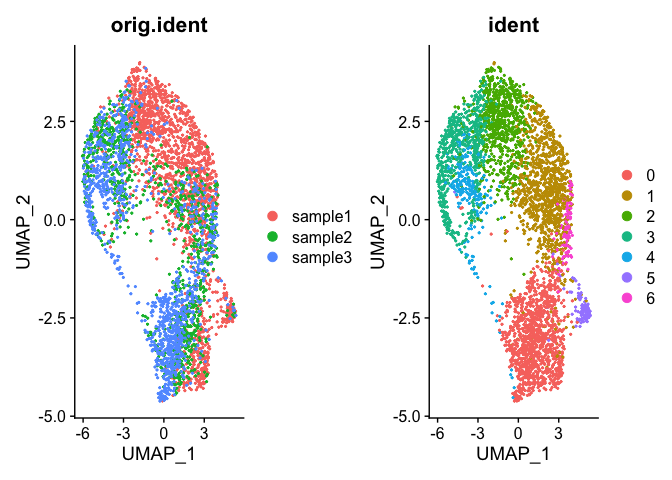
DimPlot(trA.integrated, group.by = c("orig.ident", "ident"))

QUESTION

How does this result look different from the result produced in the velocity section?

Setting up monocle3 cell_data_set object using the SueratWrappers

monocle3 uses a cell_data_set object, the as.cell_data_set function from SeuratWrappers can be used to “convert” a Seurat object to Monocle object. Moving the data calculated in Seurat to the appropriate slots in the Monocle object.

For trajectory analysis, ‘partitions’ as well as ‘clusters’ are needed and so the Monocle cluster_cells function must also be performed. Monocle’s clustering technique is more of a community based algorithm and actually uses the uMap plot (sort of) in its routine and partitions are more well separated groups using a statistical test from Alex Wolf et al,

cds <- as.cell_data_set(trA.integrated)
cds <- cluster_cells(cds, resolution=1e-3)

p1 <- plot_cells(cds, color_cells_by = "cluster", show_trajectory_graph = FALSE)
p2 <- plot_cells(cds, color_cells_by = "partition", show_trajectory_graph = FALSE)
wrap_plots(p1, p2)

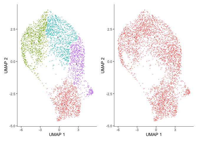
Spend a moment looking at the cell_data_set object and its slots (using slotNames) as well as cluster_cells. Try updating the resolution parameter to generate more clusters (try 1e-5, 1e-3, 1e-1, and 0).

How many clusters are generated at each level?

Subsetting partitions

Because partitions are high level separations of the data (yes we have only 1 here). It may make sense to then perform trajectory analysis on each partition separately. To do this we sould go back to Seurat, subset by partition, then back to a CDS

integrated.sub <- subset(as.Seurat(cds, assay = NULL), monocle3_partitions == 1)
cds <- as.cell_data_set(integrated.sub)

Using existing Monocle 3 cluster membership and partitions

Trajectory analysis

In a data set like this one, cells were not harvested in a time series, but may not have all been at the same developmental stage. Monocle offers trajectory analysis to model the relationships between groups of cells as a trajectory of gene expression changes. The first step in trajectory analysis is the learn_graph() function. This may be time consuming.

cds <- learn_graph(cds, use_partition = TRUE, verbose = FALSE)

After learning the graph, monocle can plot add the trajectory graph to the cell plot.

plot_cells(cds,
           color_cells_by = "cluster",
           label_groups_by_cluster=FALSE,
           label_leaves=FALSE,
           label_branch_points=FALSE)

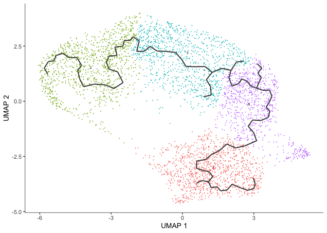
Not all of our trajectories are connected. In fact, only clusters that belong to the same partition are connected by a trajectory.

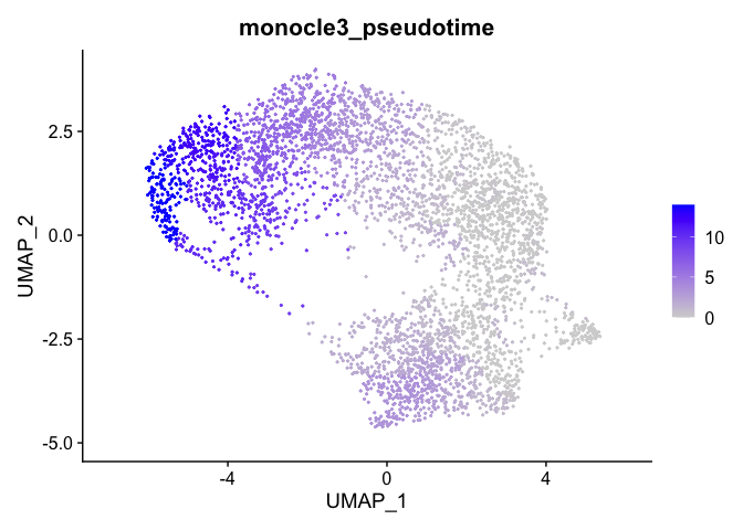
Color cells by pseudotime

We can set the root to any one of our clusters by selecting the cells in that cluster to use as the root in the function order_cells. All cells that cannot be reached from a trajectory with our selected root will be gray, which represents “infinite” pseudotime.

cds <- order_cells(cds, root_cells = colnames(cds[,clusters(cds) == 4]))
plot_cells(cds,
           color_cells_by = "pseudotime",
           group_cells_by = "cluster",
           label_cell_groups = FALSE,
           label_groups_by_cluster=FALSE,
           label_leaves=FALSE,
           label_branch_points=FALSE,
           label_roots = FALSE,
           trajectory_graph_color = "grey60")

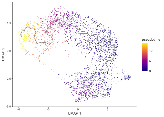
Here the pseudotime trajectory is rooted in cluster 5. This choice was arbitrary. In reality, you would make the decision about where to root your trajectory based upon what you know about your experiment. If, for example, the markers identified with cluster 1 suggest to you that cluster 1 represents the earliest developmental time point, you would likely root your pseudotime trajectory there. Explore what the pseudotime analysis looks like with the root in different clusters. Because we have not set a seed for the random process of clustering, cluster numbers will differ between R sessions.

We can export this data to the Seurat object and visualize

integrated.sub <- as.Seurat(cds, assay = NULL)
FeaturePlot(integrated.sub, "monocle3_pseudotime")

Identify genes that change as a function of pseudotime

Monocle’s graph_test() function detects genes that vary over a trajectory. This may run very slowly. Adjust the number of cores as needed.

cds_graph_test_results <- graph_test(cds,
                                     neighbor_graph = "principal_graph",
                                     cores = 8)

You may have an issue with this function in newer version of R an rBind Error.
Can fix this by:
- trace(‘calculateLW’, edit = T, where = asNamespace(“monocle3”))
- find Matrix::rBind and replace with rbind then save.

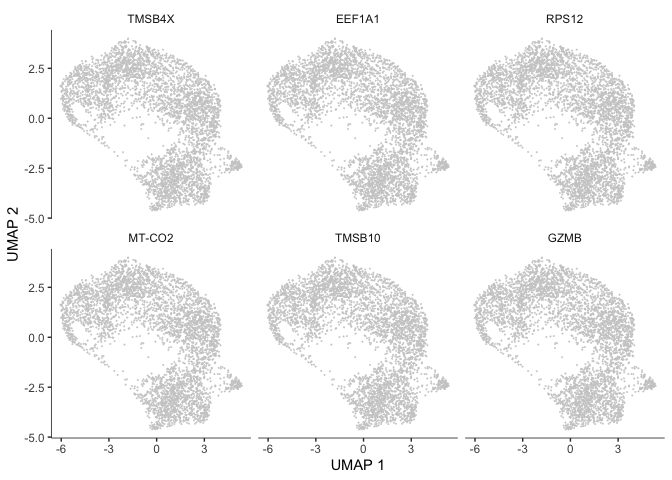
The output of this function is a table. We can look at the expression of some of these genes overlaid on the trajectory plot.

rowData(cds)$gene_short_name <- row.names(rowData(cds))

head(cds_graph_test_results, error=FALSE, message=FALSE, warning=FALSE)

deg_ids <- rownames(subset(cds_graph_test_results[order(cds_graph_test_results$morans_I, decreasing = TRUE),], q_value < 0.05))

plot_cells(cds,
           genes=head(deg_ids),
           show_trajectory_graph = FALSE,
           label_cell_groups = FALSE,
           label_leaves = FALSE)

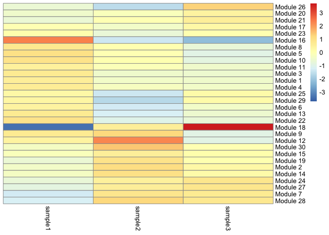
We can also calculate modules of co-expressed genes. By providing the module-finding function with a list of possible resolutions, we are telling Louvain to perform the clustering at each resolution and select the result with the greatest modularity. Modules will only be calculated for genes that vary as a function of pseudotime.

This heatmap displays the association of each gene module with each cell type.

gene_modules <- find_gene_modules(cds[deg_ids,],
                                  resolution=c(10^seq(-6,-1)))
table(gene_modules$module)

1 2 3 4 5 6 7 8 9 10 11 12 13 14 15 16 17 18 19 20 21 22 23 24 25 26 70 70 69 64 60 56 55 54 54 50 49 48 47 45 44 43 40 40 39 39 39 35 32 32 29 29 27 28 29 30 28 27 27 17

cell_groups <- data.frame(cell = row.names(colData(cds)),
                             cell_group = colData(cds)$orig.ident)
agg_mat <- aggregate_gene_expression(cds,
                                     gene_group_df = gene_modules,
                                     cell_group_df = cell_groups)
dim(agg_mat)

[1] 30 3

row.names(agg_mat) <- paste0("Module ", row.names(agg_mat))
pheatmap::pheatmap(agg_mat,
                   scale="column",
                   treeheight_row = 0,
                   treeheight_col = 0,
                   clustering_method="ward.D2")

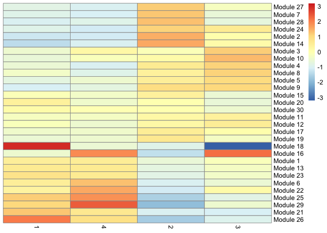
We can also display the relationship between gene modules and monocle clusters as a heatmap.

cluster_groups <- data.frame(cell = row.names(colData(cds)),
                             cluster_group = cds@clusters$UMAP[[2]])
agg_mat2 <- aggregate_gene_expression(cds, gene_modules, cluster_groups)
dim(agg_mat2)

[1] 30 4

row.names(agg_mat2) <- paste0("Module ", row.names(agg_mat2))
pheatmap::pheatmap(agg_mat2,
                   scale="column",
                   treeheight_row = 0,
                   treeheight_col = 0,
                   clustering_method="ward.D2")

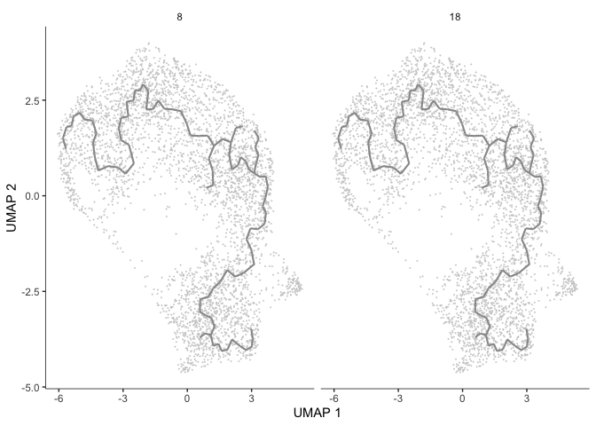
gm <- gene_modules[which(gene_modules$module %in% c(8, 18)),]
plot_cells(cds,
           genes=gm,
           label_cell_groups=FALSE,
           show_trajectory_graph=TRUE,
           label_branch_points = FALSE,
           label_roots = FALSE,
           label_leaves = FALSE,
           trajectory_graph_color = "grey60")

Warning: `guides( = FALSE)` is deprecated. Please use `guides( = "none")` instead. </div> ![](/2021-August-Advanced-Topics-in-Single-Cell-RNA-Seq-Trajectory-and-Velocity/data_analysis/monocle_files/figure-html/plotmodules-1.png) # R session information ```r sessionInfo() ```

R version 4.1.0 (2021-05-18) Platform: x86_64-apple-darwin17.0 (64-bit) Running under: macOS Big Sur 10.16 Matrix products: default BLAS: /Library/Frameworks/R.framework/Versions/4.1/Resources/lib/libRblas.dylib LAPACK: /Library/Frameworks/R.framework/Versions/4.1/Resources/lib/libRlapack.dylib locale: [1] en_US.UTF-8/en_US.UTF-8/en_US.UTF-8/C/en_US.UTF-8/en_US.UTF-8 attached base packages: [1] stats4 parallel stats graphics grDevices utils datasets [8] methods base other attached packages: [1] patchwork_1.1.1 SeuratWrappers_0.3.0 [3] SeuratObject_4.0.2 Seurat_4.0.3 [5] monocle3_1.0.0 SingleCellExperiment_1.14.1 [7] SummarizedExperiment_1.22.0 GenomicRanges_1.44.0 [9] GenomeInfoDb_1.28.1 IRanges_2.26.0 [11] S4Vectors_0.30.0 MatrixGenerics_1.4.2 [13] matrixStats_0.60.0 Biobase_2.52.0 [15] BiocGenerics_0.38.0 loaded via a namespace (and not attached): [1] plyr_1.8.6 igraph_1.2.6 lazyeval_0.2.2 [4] sp_1.4-5 splines_4.1.0 listenv_0.8.0 [7] scattermore_0.7 ggplot2_3.3.5 digest_0.6.27 [10] htmltools_0.5.1.1 viridis_0.6.1 gdata_2.18.0 [13] fansi_0.5.0 magrittr_2.0.1 tensor_1.5 [16] cluster_2.1.2 ROCR_1.0-11 remotes_2.4.0 [19] globals_0.14.0 gmodels_2.18.1 R.utils_2.10.1 [22] spatstat.sparse_2.0-0 colorspace_2.0-2 ggrepel_0.9.1 [25] xfun_0.25 dplyr_1.0.7 crayon_1.4.1 [28] RCurl_1.98-1.4 jsonlite_1.7.2 spatstat.data_2.1-0 [31] survival_3.2-12 zoo_1.8-9 glue_1.4.2 [34] polyclip_1.10-0 gtable_0.3.0 zlibbioc_1.38.0 [37] XVector_0.32.0 leiden_0.3.9 DelayedArray_0.18.0 [40] future.apply_1.8.1 abind_1.4-5 scales_1.1.1 [43] pheatmap_1.0.12 DBI_1.1.1 miniUI_0.1.1.1 [46] Rcpp_1.0.7 spData_0.3.10 viridisLite_0.4.0 [49] xtable_1.8-4 units_0.7-2 reticulate_1.20 [52] spatstat.core_2.3-0 spdep_1.1-8 proxy_0.4-26 [55] bit_4.0.4 rsvd_1.0.5 htmlwidgets_1.5.3 [58] httr_1.4.2 RColorBrewer_1.1-2 ellipsis_0.3.2 [61] ica_1.0-2 farver_2.1.0 pkgconfig_2.0.3 [64] R.methodsS3_1.8.1 sass_0.4.0 uwot_0.1.10 [67] deldir_0.2-10 utf8_1.2.2 tidyselect_1.1.1 [70] labeling_0.4.2 rlang_0.4.11 reshape2_1.4.4 [73] later_1.3.0 pbmcapply_1.5.0 munsell_0.5.0 [76] tools_4.1.0 generics_0.1.0 ggridges_0.5.3 [79] evaluate_0.14 stringr_1.4.0 fastmap_1.1.0 [82] yaml_2.2.1 goftest_1.2-2 knitr_1.33 [85] bit64_4.0.5 fitdistrplus_1.1-5 purrr_0.3.4 [88] RANN_2.6.1 pbapply_1.4-3 future_1.21.0 [91] nlme_3.1-152 mime_0.11 slam_0.1-48 [94] grr_0.9.5 R.oo_1.24.0 hdf5r_1.3.3 [97] compiler_4.1.0 plotly_4.9.4.1 png_0.1-7 [100] e1071_1.7-8 spatstat.utils_2.2-0 tibble_3.1.3 [103] bslib_0.2.5.1 stringi_1.7.3 highr_0.9 [106] RSpectra_0.16-0 lattice_0.20-44 Matrix_1.3-4 [109] classInt_0.4-3 vctrs_0.3.8 LearnBayes_2.15.1 [112] pillar_1.6.2 lifecycle_1.0.0 BiocManager_1.30.16 [115] spatstat.geom_2.2-2 lmtest_0.9-38 jquerylib_0.1.4 [118] RcppAnnoy_0.0.19 data.table_1.14.0 cowplot_1.1.1 [121] bitops_1.0-7 irlba_2.3.3 Matrix.utils_0.9.8 [124] raster_3.4-13 httpuv_1.6.2 R6_2.5.1 [127] promises_1.2.0.1 KernSmooth_2.23-20 gridExtra_2.3 [130] parallelly_1.27.0 codetools_0.2-18 gtools_3.9.2 [133] boot_1.3-28 MASS_7.3-54 assertthat_0.2.1 [136] leidenbase_0.1.3 sctransform_0.3.2 GenomeInfoDbData_1.2.6 [139] expm_0.999-6 mgcv_1.8-36 grid_4.1.0 [142] rpart_4.1-15 coda_0.19-4 class_7.3-19 [145] tidyr_1.1.3 rmarkdown_2.10 Rtsne_0.15 [148] sf_1.0-2 shiny_1.6.0

☰ Menu

Adv Topics in scRNA-Seq: Trajectory and Velocity Analysis

Trajectory Analysis with Monocle 3

Project set-up

Loading data into Seurat

Seurat processing of data

Setting up monocle3 cell_data_set object using the SueratWrappers

Subsetting partitions

Trajectory analysis

Color cells by pseudotime

Identify genes that change as a function of pseudotime