
Last Updated: March 23 2021, 5pm
Part 2: Some QA/QC, filtering and normalization
Load libraries
library(Seurat)
library(biomaRt)
library(ggplot2)
library(knitr)
library(kableExtra)
Load the Seurat object from part 1
load(file="original_seurat_object.RData")
experiment.aggregate
set.seed(12345)
Some basic QA/QC of the metadata, print tables of the 5% quantiles.
Show 5% quantiles for number of genes per cell per sample
kable(do.call("cbind", tapply(experiment.aggregate$nFeature_RNA,
                      Idents(experiment.aggregate),quantile,probs=seq(0,1,0.05))),
      caption = "5% Quantiles of Genes/Cell by Sample") %>% kable_styling()
| PBMC2 | PBMC3 | T021PBMC | T022PBMC | |
|---|---|---|---|---|
| 0% | 300.0 | 300.00 | 300.0 | 300.00 |
| 5% | 311.0 | 364.00 | 445.0 | 618.35 |
| 10% | 321.0 | 459.30 | 598.0 | 884.40 |
| 15% | 334.0 | 563.00 | 808.0 | 1181.20 |
| 20% | 347.0 | 678.60 | 1030.0 | 1356.40 |
| 25% | 365.0 | 825.00 | 1190.0 | 1452.00 |
| 30% | 393.0 | 969.90 | 1276.0 | 1527.00 |
| 35% | 439.0 | 1091.00 | 1334.0 | 1588.00 |
| 40% | 509.0 | 1207.00 | 1390.0 | 1646.00 |
| 45% | 613.0 | 1312.00 | 1438.0 | 1695.00 |
| 50% | 697.0 | 1412.00 | 1481.0 | 1741.00 |
| 55% | 772.0 | 1521.65 | 1528.0 | 1788.85 |
| 60% | 842.0 | 1629.80 | 1573.0 | 1843.00 |
| 65% | 920.0 | 1753.00 | 1620.0 | 1894.55 |
| 70% | 1000.0 | 1883.10 | 1668.3 | 1950.90 |
| 75% | 1100.0 | 2022.00 | 1726.0 | 2021.00 |
| 80% | 1211.0 | 2212.00 | 1802.0 | 2114.00 |
| 85% | 1327.0 | 2395.00 | 1905.0 | 2252.95 |
| 90% | 1473.0 | 2641.00 | 2075.1 | 2508.00 |
| 95% | 1717.7 | 2997.70 | 2451.0 | 3013.25 |
| 100% | 6260.0 | 6303.00 | 5145.0 | 6407.00 |
Show 5% quantiles for number of UMI per cell per sample
kable(do.call("cbind", tapply(experiment.aggregate$nCount_RNA,
                                      Idents(experiment.aggregate),quantile,probs=seq(0,1,0.05))),
      caption = "5% Quantiles of UMI/Cell by Sample") %>% kable_styling()
| PBMC2 | PBMC3 | T021PBMC | T022PBMC | |
|---|---|---|---|---|
| 0% | 364.00 | 387.00 | 408.00 | 415.00 |
| 5% | 431.00 | 616.15 | 700.00 | 1068.40 |
| 10% | 455.00 | 797.00 | 1020.00 | 1673.40 |
| 15% | 482.00 | 1008.00 | 1514.00 | 2617.15 |
| 20% | 513.00 | 1287.00 | 2235.00 | 3268.20 |
| 25% | 556.25 | 1640.25 | 2808.00 | 3648.75 |
| 30% | 630.00 | 2024.00 | 3135.00 | 3923.10 |
| 35% | 745.55 | 2389.05 | 3348.00 | 4157.45 |
| 40% | 894.00 | 2743.40 | 3520.00 | 4363.80 |
| 45% | 1035.00 | 3066.35 | 3682.05 | 4559.15 |
| 50% | 1156.00 | 3398.50 | 3830.00 | 4752.00 |
| 55% | 1286.00 | 3784.65 | 3973.00 | 4930.85 |
| 60% | 1451.00 | 4210.80 | 4125.40 | 5121.20 |
| 65% | 1659.00 | 4684.95 | 4293.85 | 5336.20 |
| 70% | 1936.10 | 5279.00 | 4483.00 | 5582.00 |
| 75% | 2315.75 | 5940.75 | 4696.50 | 5847.25 |
| 80% | 2810.00 | 6852.80 | 4989.00 | 6211.20 |
| 85% | 3373.15 | 7873.65 | 5468.30 | 6772.75 |
| 90% | 3905.40 | 9212.70 | 6174.10 | 7907.60 |
| 95% | 4857.35 | 11522.20 | 7717.55 | 10940.50 |
| 100% | 53960.00 | 45925.00 | 40004.00 | 65032.00 |
Show 5% quantiles for number of mitochondrial percentage per cell per sample
kable(round(do.call("cbind", tapply(experiment.aggregate$percent.mito, Idents(experiment.aggregate),quantile,probs=seq(0,1,0.05))), digits = 3),
      caption = "5% Quantiles of Percent Mitochondria by Sample") %>% kable_styling()
| PBMC2 | PBMC3 | T021PBMC | T022PBMC | |
|---|---|---|---|---|
| 0% | 0.000 | 0.000 | 0.000 | 0.000 |
| 5% | 0.170 | 0.901 | 1.297 | 0.857 |
| 10% | 0.433 | 1.193 | 1.544 | 1.025 |
| 15% | 0.760 | 1.450 | 1.736 | 1.137 |
| 20% | 1.107 | 1.627 | 1.894 | 1.247 |
| 25% | 1.452 | 1.811 | 2.033 | 1.341 |
| 30% | 1.795 | 1.996 | 2.183 | 1.431 |
| 35% | 2.144 | 2.187 | 2.317 | 1.523 |
| 40% | 2.560 | 2.376 | 2.450 | 1.609 |
| 45% | 3.045 | 2.577 | 2.583 | 1.700 |
| 50% | 3.598 | 2.795 | 2.731 | 1.798 |
| 55% | 4.193 | 3.010 | 2.893 | 1.902 |
| 60% | 4.878 | 3.268 | 3.060 | 2.028 |
| 65% | 5.556 | 3.548 | 3.261 | 2.167 |
| 70% | 6.326 | 3.865 | 3.505 | 2.337 |
| 75% | 7.135 | 4.287 | 3.810 | 2.560 |
| 80% | 8.255 | 4.831 | 4.220 | 2.841 |
| 85% | 9.867 | 5.667 | 4.785 | 3.369 |
| 90% | 13.351 | 7.015 | 5.807 | 4.363 |
| 95% | 19.802 | 9.943 | 8.575 | 7.221 |
| 100% | 66.956 | 64.033 | 58.654 | 64.962 |
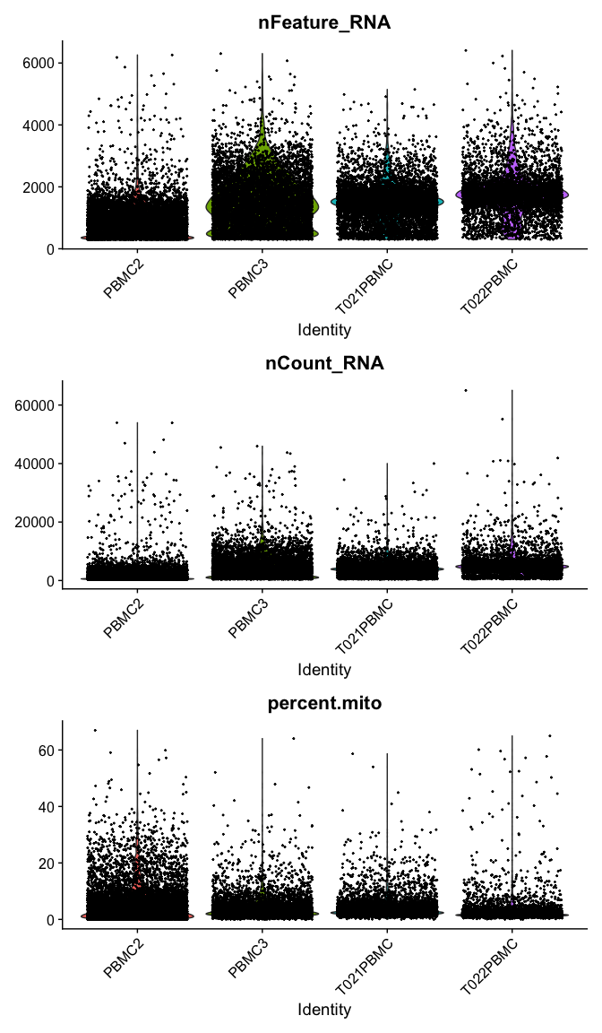
Violin plot of 1) number of genes, 2) number of UMI and 3) percent mitochondrial genes
VlnPlot(
  experiment.aggregate,
  features = c("nFeature_RNA", "nCount_RNA","percent.mito"),
  ncol = 1, pt.size = 0.3)
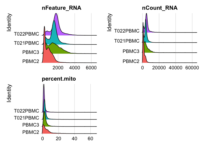
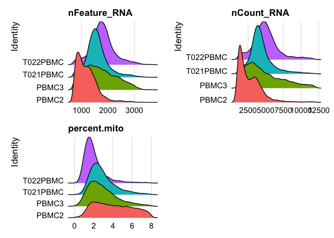
plot ridgeplots of the same data
RidgePlot(experiment.aggregate, features=c("nFeature_RNA","nCount_RNA", "percent.mito"), ncol = 2)
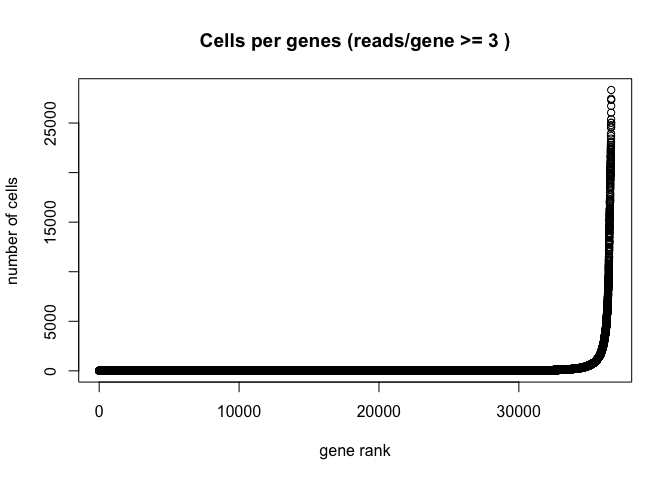
Plot the distribution of number of cells each gene is represented by
plot(sort(Matrix::rowSums(GetAssayData(experiment.aggregate) >= 3)) , xlab="gene rank", ylab="number of cells", main="Cells per genes (reads/gene >= 3 )")
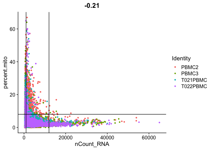
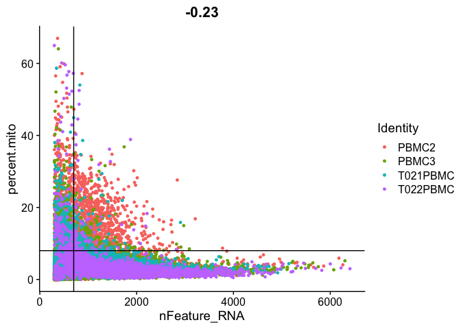
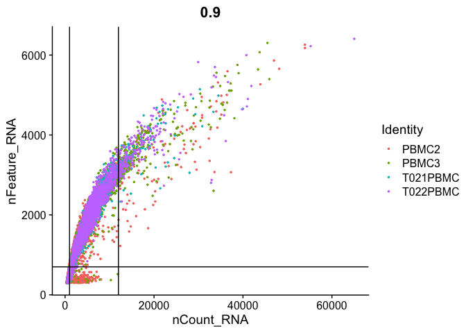
Gene Plot, scatter plot of gene expression across cells, (colored by sample), drawing horizontal an verticale lines at proposed filtering cutoffs.
FeatureScatter(experiment.aggregate, feature1 = "nCount_RNA", feature2 = "percent.mito") + geom_vline(xintercept = c(1000,12000)) + geom_hline(yintercept = 8)
FeatureScatter(experiment.aggregate, feature1 = "nFeature_RNA", feature2 = "percent.mito") + geom_vline(xintercept = 700) + geom_hline(yintercept = 8)
FeatureScatter(
  experiment.aggregate, "nCount_RNA", "nFeature_RNA",
  pt.size = 0.5)  + geom_vline(xintercept = c(1000,12000)) + geom_hline(yintercept = 700)
Cell filtering
We use the information above to filter out cells. Here we choose those that have percent mitochondrial genes max of 8%, unique UMI counts under 1,000 or greater than 12,000 and contain at least 700 features within them.
table(experiment.aggregate$orig.ident)
experiment.aggregate <- subset(experiment.aggregate, percent.mito <= 8)

experiment.aggregate <- subset(experiment.aggregate, nCount_RNA >= 1000 & nCount_RNA <= 12000)

experiment.aggregate <- subset(experiment.aggregate, nFeature_RNA >= 700)

experiment.aggregate
table(experiment.aggregate$orig.ident)
Lets se the ridgeplots now after filtering
RidgePlot(experiment.aggregate, features=c("nFeature_RNA","nCount_RNA", "percent.mito"), ncol = 2)
You may also want to filter out additional genes.
When creating the base Seurat object we did filter out some genes, recall Keep all genes expressed in >= 10 cells. After filtering cells and you may want to be more aggressive with the gene filter. Seurat doesn’t supply such a function (that I can find), so below is a function that can do so, it filters genes requiring a min.value (log-normalized) in at least min.cells, here expression of 1 in at least 400 cells.
experiment.aggregate
FilterGenes <-
 function (object, min.value=1, min.cells = 0, genes = NULL) {
   genes.use <- rownames(object)
   if (!is.null(genes)) {
     genes.use <- intersect(genes.use, genes)
     object@data <- GetAssayData(object)[genes.use, ]
   } else if (min.cells > 0) {
     num.cells <- Matrix::rowSums(GetAssayData(object) > min.value)
     genes.use <- names(num.cells[which(num.cells >= min.cells)])
     object = object[genes.use, ]
   }
  object <- LogSeuratCommand(object = object)
  return(object)
}

experiment.aggregate.genes <- FilterGenes(object = experiment.aggregate, min.value = 1, min.cells = 400)
experiment.aggregate.genes
rm(experiment.aggregate.genes)
FOR THIS WORKSHOP ONLY: Lets reduce the dataset down to 1000 cells per sample for time
table(Idents(experiment.aggregate))
experiment.aggregate <- experiment.aggregate[,unlist(sapply(split(seq_along(Cells(experiment.aggregate)), experiment.aggregate$orig.ident), sample, size=1000, simplify = F))]
table(Idents(experiment.aggregate))
Next we want to normalize the data
After filtering out cells from the dataset, the next step is to normalize the data. By default, we employ a global-scaling normalization method LogNormalize that normalizes the gene expression measurements for each cell by the total expression, multiplies this by a scale factor (10,000 by default), and then log-transforms the data.
?NormalizeData
experiment.aggregate <- NormalizeData(
  object = experiment.aggregate,
  normalization.method = "LogNormalize",
  scale.factor = 10000)
Calculate Cell-Cycle with Seurat, the list of genes comes with Seurat (only for human)
Dissecting the multicellular ecosystem of metastatic melanoma by single-cell RNA-seq
First need to convert to mouse symbols, we’ll use Biomart for that too.
# Mouse Code
# convertHumanGeneList <- function(x){
#   require("biomaRt")
#   human = useEnsembl("ensembl", dataset = "hsapiens_gene_ensembl", mirror = "uswest")
#   mouse = useEnsembl("ensembl", dataset = "mmusculus_gene_ensembl", mirror = "uswest")
#
#   genes = getLDS(attributes = c("hgnc_symbol"), filters = "hgnc_symbol", values = x , mart = human, attributesL = c("mgi_symbol"), martL = mouse, uniqueRows=T)
#
#   humanx <- unique(genes[, 2])
#
#   # Print the first 6 genes found to the screen
#   print(head(humanx))
#   return(humanx)
# }
#
# m.s.genes <- convertHumanGeneList(cc.genes.updated.2019$s.genes)
# m.g2m.genes <- convertHumanGeneList(cc.genes.updated.2019$g2m.genes)
#
# # Create our Seurat object and complete the initialization steps
# experiment.aggregate <- CellCycleScoring(experiment.aggregate, s.features = m.s.genes, g2m.features = m.g2m.genes, set.ident = TRUE)

# Human Code
s.genes <- (cc.genes$s.genes)
g2m.genes <- (cc.genes$g2m.genes)

# Create our Seurat object and complete the initialization steps
experiment.aggregate <- CellCycleScoring(experiment.aggregate, s.features = s.genes, g2m.features = g2m.genes, set.ident = TRUE)
Table of cell cycle (seurate)
table(experiment.aggregate@meta.data$Phase) %>% kable(caption = "Number of Cells in each Cell Cycle Stage", col.names = c("Stage", "Count"), align = "c") %>% kable_styling()
| Stage | Count |
|---|---|
| G1 | 1676 |
| G2M | 898 |
| S | 1426 |
Fixing the defualt “Ident” in Seurat
table(Idents(experiment.aggregate))
## So lets change it back to samplename
Idents(experiment.aggregate) <- "orig.ident"
table(Idents(experiment.aggregate))
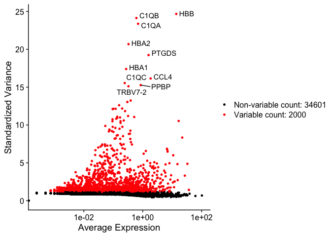
Identify variable genes
The function FindVariableFeatures identifies the most highly variable genes (default 2000 genes) by fitting a line to the relationship of log(variance) and log(mean) using loess smoothing, uses this information to standardize the data, then calculates the variance of the standardized data. This helps avoid selecting genes that only appear variable due to their expression level.
?FindVariableFeatures
experiment.aggregate <- FindVariableFeatures(
  object = experiment.aggregate,
  selection.method = "vst")

length(VariableFeatures(experiment.aggregate))
top10 <- head(VariableFeatures(experiment.aggregate), 10)

top10
vfp1 <- VariableFeaturePlot(experiment.aggregate)
vfp1 <- LabelPoints(plot = vfp1, points = top10, repel = TRUE)
vfp1
Instead of using the variable genes function, lets instead assign to variable genes to a set of “minimally expressed” genes.
dim(experiment.aggregate)
min.value = 2
min.cells = 10
num.cells <- Matrix::rowSums(GetAssayData(experiment.aggregate, slot = "count") > min.value)
genes.use <- names(num.cells[which(num.cells >= min.cells)])
length(genes.use)
VariableFeatures(experiment.aggregate) <- genes.use
Question(s)
- Play some with the filtering parameters, see how results change?
- How do the results change if you use selection.method = “dispersion” or selection.method = “mean.var.plot”
Finally, lets save the filtered and normalized data
save(experiment.aggregate, file="pre_sample_corrected.RData")
Get the next Rmd file
download.file("https://raw.githubusercontent.com/ucdavis-bioinformatics-training/2021-August-Single-Cell-RNA-Seq-Analysis/master/data_analysis/scRNA_Workshop-PART3.Rmd", "scRNA_Workshop-PART3.Rmd")
Session Information
sessionInfo()