
Setup additinal options
Load libraries
library(Seurat)
library(ggplot2)
library(limma)
library(topGO)
library(WGCNA)
Load the Seurat object
load("clusters_seurat_object.RData")
experiment.merged
An object of class Seurat
36601 features across 4000 samples within 1 assay
Active assay: RNA (36601 features, 3783 variable features)
3 dimensional reductions calculated: pca, tsne, umap
Idents(experiment.merged) <- "RNA_snn_res.0.25"
2. Gene Ontology (GO) Enrichment of Genes Expressed in a Cluster
# install org.Hs.eg.db from Bioconductor if not already installed (for mouse only)
cluster0 <- subset(experiment.merged, idents = '0')
expr <- as.matrix(GetAssayData(cluster0))
# Filter out genes that are 0 for every cell in this cluster
bad <- which(rowSums(expr) == 0)
expr <- expr[-bad,]

# Select genes that are expressed > 0 in at least 75% of cells (somewhat arbitrary definition)
n.gt.0 <- apply(expr, 1, function(x)length(which(x > 0)))
expressed.genes <- rownames(expr)[which(n.gt.0/ncol(expr) >= 0.5)]
all.genes <- rownames(expr)

# define geneList as 1 if gene is in expressed.genes, 0 otherwise
geneList <- ifelse(all.genes %in% expressed.genes, 1, 0)
names(geneList) <- all.genes

# Create topGOdata object
	GOdata <- new("topGOdata",
		ontology = "BP", # use biological process ontology
		allGenes = geneList,
		geneSelectionFun = function(x)(x == 1),
              annot = annFUN.org, mapping = "org.Hs.eg.db", ID = "symbol")
# Test for enrichment using Fisher's Exact Test
	resultFisher <- runTest(GOdata, algorithm = "elim", statistic = "fisher")
	GenTable(GOdata, Fisher = resultFisher, topNodes = 20, numChar = 60)
GO.ID Term Annotated Significant Expected Fisher
1 GO:0006614 SRP-dependent cotranslational protein targeting to membrane 95 80 5.35 < 1e-30
2 GO:0006413 translational initiation 184 101 10.36 < 1e-30
3 GO:0000184 nuclear-transcribed mRNA catabolic process, nonsense-mediate... 119 81 6.70 < 1e-30
4 GO:0019083 viral transcription 173 81 9.74 < 1e-30
5 GO:0002181 cytoplasmic translation 92 49 5.18 1.0e-28
6 GO:0035722 interleukin-12-mediated signaling pathway 43 20 2.42 2.2e-14
7 GO:0060337 type I interferon signaling pathway 74 24 4.17 8.3e-13
8 GO:0006123 mitochondrial electron transport, cytochrome c to oxygen 15 10 0.84 6.9e-10
9 GO:0016032 viral process 744 167 41.88 2.4e-09
10 GO:0042776 mitochondrial ATP synthesis coupled proton transport 21 11 1.18 3.5e-09
11 GO:0000027 ribosomal large subunit assembly 27 12 1.52 7.3e-09
12 GO:0000381 regulation of alternative mRNA splicing, via spliceosome 53 16 2.98 1.8e-08
13 GO:0043066 negative regulation of apoptotic process 621 78 34.96 6.0e-08
14 GO:0043312 neutrophil degranulation 421 52 23.70 6.4e-08
15 GO:0002479 antigen processing and presentation of exogenous peptide ant... 71 17 4.00 2.8e-07
16 GO:0006364 rRNA processing 206 36 11.60 3.9e-07
17 GO:0000398 mRNA splicing, via spliceosome 312 54 17.56 4.6e-07
18 GO:0002480 antigen processing and presentation of exogenous peptide ant... 8 6 0.45 7.9e-07
19 GO:0001732 formation of cytoplasmic translation initiation complex 16 8 0.90 8.3e-07
20 GO:0000028 ribosomal small subunit assembly 16 8 0.90 8.3e-07
- Annotated: number of genes (out of all.genes) that are annotated with that GO term
- Significant: number of genes that are annotated with that GO term and meet our criteria for “expressed”
- Expected: Under random chance, number of genes that would be expected to be annotated with that GO term and meeting our criteria for “expressed”
- Fisher: (Raw) p-value from Fisher’s Exact Test
#3. Weighted Gene Co-Expression Network Analysis (WGCNA) WGCNA identifies groups of genes (“modules”) with correlated expression. WARNING: TAKES A LONG TIME TO RUN
options(stringsAsFactors = F)
datExpr <- t(as.matrix(GetAssayData(experiment.merged)))[,VariableFeatures(experiment.merged)]  # only use variable genes in analysis

net <- blockwiseModules(datExpr, power = 10,
  corType = "bicor", # use robust correlation
	networkType = "signed", minModuleSize = 10,
	reassignThreshold = 0, mergeCutHeight = 0.15,
	numericLabels = F, pamRespectsDendro = FALSE,
	saveTOMs = TRUE,
	saveTOMFileBase = "TOM",
	verbose = 3)
Calculating module eigengenes block-wise from all genes
Flagging genes and samples with too many missing values...
..step 1
..Working on block 1 .
TOM calculation: adjacency..
..will not use multithreading.
Fraction of slow calculations: 0.000000
..connectivity..
..matrix multiplication (system BLAS)..
..normalization..
..done.
..saving TOM for block 1 into file TOM-block.1.RData
....clustering..
....detecting modules..
....calculating module eigengenes..
....checking kME in modules..
..removing 599 genes from module 1 because their KME is too low.
..removing 65 genes from module 2 because their KME is too low.
..removing 48 genes from module 4 because their KME is too low.
..removing 7 genes from module 6 because their KME is too low.
..merging modules that are too close..
mergeCloseModules: Merging modules whose distance is less than 0.15
Calculating new MEs...
table(net$colors)
blue brown grey turquoise yellow
71 46 3463 192 11
# Convert labels to colors for plotting
mergedColors = net$colors
# Plot the dendrogram and the module colors underneath
plotDendroAndColors(net$dendrograms[[1]], mergedColors[net$blockGenes[[1]]],
"Module colors",
dendroLabels = FALSE, hang = 0.03,
addGuide = TRUE, guideHang = 0.05)
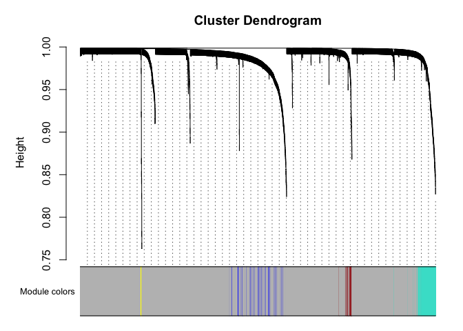 Genes in grey module are unclustered.
What genes are in the “blue” module?
colnames(datExpr)[net$colors == "blue"]
[1] "ISG15" "EFHD2" "SH3BGRL3" "FGR" "IFI6" "GNG5" "S100A10" "S100A11" "S100A6" "S100A4" "TPM3" "FCER1G" "ARPC5" "H3F3A" "ID2" "PLEK" "TMSB10" "VAMP8" "DBI" "RHOA" "PLAC8" "ATP6V0E1" "PRELID1" "CLIC1" "PSMB9" "ACTB" "RAC1" "ARPC1B" "ATP5MF" "GNB2" "LY6E" "SEC61B" "MAP3K8" "SRGN" "IFITM2" "IFITM3" "POLR2L" "CTSD" "RHOG" "UBE2L6"
[41] "COX8A" "CFL1" "GSTP1" "CARD16" "GAPDH" "TPI1" "BLOC1S1" "CD63" "MYL6" "ARPC3" "PSME2" "SERF2" "ANXA2" "ELOB" "MT2A" "PSMB10" "CYBA" "PFN1" "GABARAP" "ACTG1" "UQCR11" "OAZ1" "WDR83OS" "BST2" "COX6B1" "TYROBP" "EMP3" "ATP5F1E" "PSMA7" "ITGB2" "LGALS1"
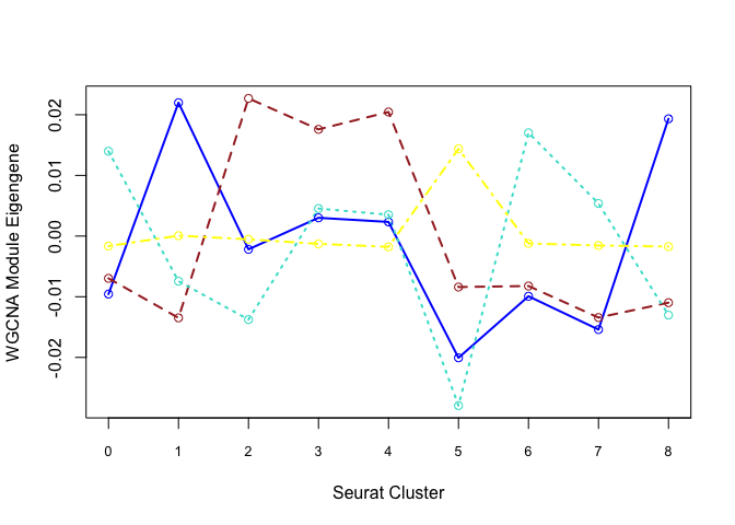
Each cluster is represented by a summary “eigengene”. Plot eigengenes for each non-grey module by clusters from Seurat:
f <- function(module){
  eigengene <- unlist(net$MEs[paste0("ME", module)])
  means <- tapply(eigengene, Idents(experiment.merged), mean, na.rm = T)
  return(means)
}
unique(net$colors)
[1] "grey" "blue" "turquoise" "brown" "yellow"
modules <- c("blue", "brown", "turquoise", "yellow")
plotdat <- sapply(modules, f)
matplot(plotdat, col = modules, type = "l", lwd = 2, xaxt = "n", xlab = "Seurat Cluster",
        ylab = "WGCNA Module Eigengene")
axis(1, at = 1:19, labels = 0:18, cex.axis = 0.8)
matpoints(plotdat, col = modules, pch = 21)
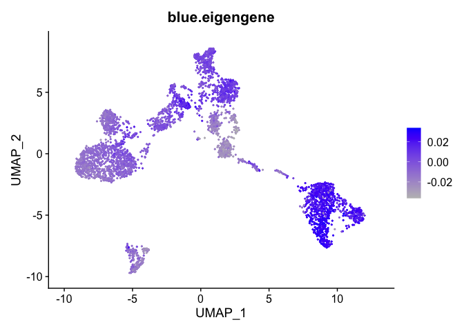
Can also plot the module onto the tsne plot
blue.eigengene <- unlist(net$MEs[paste0("ME", "blue")])
names(blue.eigengene) <- rownames(datExpr)
experiment.merged$blue.eigengene <- blue.eigengene
FeaturePlot(experiment.merged, features = "blue.eigengene", cols = c("grey", "blue"))
Session Information
sessionInfo()
R version 4.0.3 (2020-10-10)
Platform: x86_64-apple-darwin17.0 (64-bit)
Running under: macOS Big Sur 10.16
Matrix products: default
BLAS: /Library/Frameworks/R.framework/Versions/4.0/Resources/lib/libRblas.dylib
LAPACK: /Library/Frameworks/R.framework/Versions/4.0/Resources/lib/libRlapack.dylib
locale:
[1] en_US.UTF-8/en_US.UTF-8/en_US.UTF-8/C/en_US.UTF-8/en_US.UTF-8
attached base packages:
[1] stats4 parallel stats graphics grDevices utils datasets methods base
other attached packages:
[1] org.Hs.eg.db_3.11.4 WGCNA_1.70-3 fastcluster_1.1.25 dynamicTreeCut_1.63-1 topGO_2.40.0 SparseM_1.81 GO.db_3.11.4 AnnotationDbi_1.50.3 IRanges_2.22.2 S4Vectors_0.26.1 Biobase_2.48.0 graph_1.66.0 BiocGenerics_0.34.0 limma_3.44.3 ggplot2_3.3.3 SeuratObject_4.0.0 Seurat_4.0.1
loaded via a namespace (and not attached):
[1] backports_1.2.1 Hmisc_4.5-0 plyr_1.8.6 igraph_1.2.6 lazyeval_0.2.2 splines_4.0.3 listenv_0.8.0 scattermore_0.7 digest_0.6.27 foreach_1.5.1 htmltools_0.5.1.1 fansi_0.4.2 checkmate_2.0.0 magrittr_2.0.1 memoise_2.0.0 tensor_1.5 cluster_2.1.1 doParallel_1.0.16 ROCR_1.0-11 globals_0.14.0
[21] matrixStats_0.58.0 spatstat.sparse_2.0-0 jpeg_0.1-8.1 colorspace_2.0-0 blob_1.2.1 ggrepel_0.9.1 xfun_0.22 dplyr_1.0.5 crayon_1.4.1 jsonlite_1.7.2 spatstat.data_2.1-0 impute_1.62.0 survival_3.2-10 zoo_1.8-9 iterators_1.0.13 glue_1.4.2 polyclip_1.10-0 gtable_0.3.0 leiden_0.3.7 future.apply_1.7.0
[41] abind_1.4-5 scales_1.1.1 DBI_1.1.1 miniUI_0.1.1.1 Rcpp_1.0.6 htmlTable_2.1.0 viridisLite_0.3.0 xtable_1.8-4 reticulate_1.18 spatstat.core_2.0-0 foreign_0.8-81 bit_4.0.4 preprocessCore_1.50.0 Formula_1.2-4 htmlwidgets_1.5.3 httr_1.4.2 RColorBrewer_1.1-2 ellipsis_0.3.1 ica_1.0-2 farver_2.1.0
[61] pkgconfig_2.0.3 nnet_7.3-15 sass_0.3.1 uwot_0.1.10 deldir_0.2-10 utf8_1.2.1 labeling_0.4.2 tidyselect_1.1.0 rlang_0.4.10 reshape2_1.4.4 later_1.1.0.1 munsell_0.5.0 tools_4.0.3 cachem_1.0.4 generics_0.1.0 RSQLite_2.2.4 ggridges_0.5.3 evaluate_0.14 stringr_1.4.0 fastmap_1.1.0
[81] yaml_2.2.1 goftest_1.2-2 knitr_1.31 bit64_4.0.5 fitdistrplus_1.1-3 purrr_0.3.4 RANN_2.6.1 pbapply_1.4-3 future_1.21.0 nlme_3.1-152 mime_0.10 rstudioapi_0.13 compiler_4.0.3 plotly_4.9.3 png_0.1-7 spatstat.utils_2.1-0 tibble_3.1.0 bslib_0.2.4 stringi_1.5.3 highr_0.8
[101] lattice_0.20-41 Matrix_1.3-2 vctrs_0.3.6 pillar_1.5.1 lifecycle_1.0.0 spatstat.geom_2.0-1 lmtest_0.9-38 jquerylib_0.1.3 RcppAnnoy_0.0.18 data.table_1.14.0 cowplot_1.1.1 irlba_2.3.3 httpuv_1.5.5 patchwork_1.1.1 latticeExtra_0.6-29 R6_2.5.0 promises_1.2.0.1 KernSmooth_2.23-18 gridExtra_2.3 parallelly_1.24.0
[121] codetools_0.2-18 MASS_7.3-53.1 assertthat_0.2.1 withr_2.4.1 sctransform_0.3.2 mgcv_1.8-34 grid_4.0.3 rpart_4.1-15 tidyr_1.1.3 rmarkdown_2.7 Rtsne_0.15 base64enc_0.1-3 shiny_1.6.0