Home
Preliminaries
Before the course
File downloads
Data Analysis
Differential Expression
Enrichment Analysis
R Code for Quizzes
Upcoming
Upcoming Bioinformatics Core Courses

Differential Gene Expression Analysis in R

Differential Gene Expression (DGE) looks for genes whose expression changes in response to treatment or between groups.

A lot of RNA-seq analysis has been done in R and so there are many packages available to analyze and view this data. Two of the most commonly used are:

DESeq2, developed by Simon Anders (also created htseq) in Wolfgang Huber’s group at EMBL
edgeR and Voom (extension to limma for RNA-seq), developed out of Gordon Smyth’s group from the Walter and Eliza Hall Institute of Medical Research in Australia

Differential Expression Analysis with limma-Voom

limma is an R package that was originally developed for differential expression (DE) analysis of gene expression microarray data.

voom is a function in the limma package that transforms RNA-Seq data for use with limma.

Together they allow fast, flexible, and powerful analyses of RNA-Seq data. Limma-voom is our tool of choice for DE analyses because it:

Allows for incredibly flexible model specification (you can include multiple categorical and continuous variables, allowing incorporation of almost any kind of metadata).
Based on simulation studies, maintains the false discovery rate at or below the nominal rate, unlike some other packages.
Empirical Bayes smoothing of gene-wise standard deviations provides increased power.

Basic Steps of Differential Gene Expression

Read count data into R
Calculate normalization factors (sample-specific adjustments for differences in e.g. read depth)
Filter genes (uninteresting genes, e.g. unexpressed)
Account for expression-dependent variability by transformation, weighting, or modeling
Fit a linear model (or generalized linear model, or nonparametric model)
Perform statistical comparisons of interest (using contrasts)
Adjust for multiple testing, Benjamini-Hochberg (BH) or q-value
Check results for confidence
Attach annotation if available and write tables

library(edgeR)
library(RColorBrewer)
library(gplots)

The dataset

The data used in the example are from Kurtulus et al. and are from mouse CD8+ T cells. We use the portion of the experiment in which they identified three T-cell subsets:

CD62L-Slamf7hiCX3CR1- (“memory precursor like”), 5 samples
CD62L-Slamf7hiCX3CR1+ (“effector like”), 3 samples
CD62LhiSlamf7-CX3CR1- (“naive like”), 6 samples

The data used in this example were obtained from SRA, preprocessed using HTStream, and aligned and counted using STAR.

The counts table

The counts table we will use for our differential expression analysis is of the following format:

One column for every sample
One row for every gene in the annotation .gtf file used for alignment
Elements are the raw counts of reads aligning to a given gene for a given sample

1. Read in the counts table and create our DGEList object

counts <- read.delim("counts_for_course.txt", row.names = 1)
head(counts)

SRR8245064 SRR8245065 SRR8245066 SRR8245067 SRR8245068 ENSMUSG00000102693.2 3 0 0 0 0 ENSMUSG00000064842.3 0 0 0 0 0 ENSMUSG00000051951.6 8 27 16 5 5 ENSMUSG00000102851.2 0 0 3 0 0 ENSMUSG00000103377.2 13 0 2 7 2 ENSMUSG00000104017.2 7 1 7 6 11 SRR8245069 SRR8245070 SRR8245071 SRR8245072 SRR8245073 ENSMUSG00000102693.2 0 1 0 0 0 ENSMUSG00000064842.3 0 0 0 0 0 ENSMUSG00000051951.6 9 6 5 2 0 ENSMUSG00000102851.2 0 0 0 0 0 ENSMUSG00000103377.2 0 0 0 0 0 ENSMUSG00000104017.2 30 5 0 0 0 SRR8245074 SRR8245075 SRR8245076 SRR8245077 ENSMUSG00000102693.2 0 0 0 3 ENSMUSG00000064842.3 0 0 0 0 ENSMUSG00000051951.6 0 0 0 1 ENSMUSG00000102851.2 0 0 0 0 ENSMUSG00000103377.2 0 0 1 0 ENSMUSG00000104017.2 2 21 0 1

Create Differential Gene Expression List Object (DGEList) object

A DGEList is an object in the package edgeR for storing count data, normalization factors, and other information

d0 <- DGEList(counts)

1a. Read in Annotation

anno <- read.delim("annotation.txt")
dim(anno)

[1] 55414 3

head(anno)

Gene.stable.ID 1 ENSMUSG00000064336 2 ENSMUSG00000064337 3 ENSMUSG00000064338 4 ENSMUSG00000064339 5 ENSMUSG00000064340 6 ENSMUSG00000064341 Gene.description 1 mitochondrially encoded tRNA phenylalanine [Source:MGI Symbol;Acc:MGI:102487] 2 mitochondrially encoded 12S rRNA [Source:MGI Symbol;Acc:MGI:102493] 3 mitochondrially encoded tRNA valine [Source:MGI Symbol;Acc:MGI:102472] 4 mitochondrially encoded 16S rRNA [Source:MGI Symbol;Acc:MGI:102492] 5 mitochondrially encoded tRNA leucine 1 [Source:MGI Symbol;Acc:MGI:102482] 6 mitochondrially encoded NADH dehydrogenase 1 [Source:MGI Symbol;Acc:MGI:101787] Gene.name 1 mt-Tf 2 mt-Rnr1 3 mt-Tv 4 mt-Rnr2 5 mt-Tl1 6 mt-Nd1

tail(anno)

Gene.stable.ID 55409 ENSMUSG00000044103 55410 ENSMUSG00000026984 55411 ENSMUSG00000104173 55412 ENSMUSG00000083172 55413 ENSMUSG00000026983 55414 ENSMUSG00000046845 Gene.description 55409 interleukin 36G [Source:MGI Symbol;Acc:MGI:2449929] 55410 interleukin 36A [Source:MGI Symbol;Acc:MGI:1859324] 55411 predicted gene, 37703 [Source:MGI Symbol;Acc:MGI:5610931] 55412 predicted gene 13409 [Source:MGI Symbol;Acc:MGI:3651609] 55413 interleukin 36 receptor antagonist [Source:MGI Symbol;Acc:MGI:1859325] 55414 interleukin 1 family, member 10 [Source:MGI Symbol;Acc:MGI:2652548] Gene.name 55409 Il36g 55410 Il36a 55411 Gm37703 55412 Gm13409 55413 Il36rn 55414 Il1f10

any(duplicated(anno$Gene.stable.ID))

[1] FALSE

1b. Read in metadata Metadata for this experiment is in a separate .csv file.

metadata <- read.csv("metadata_for_course.csv")
head(metadata)

Run Cell_type simplified_cell_type 1 SRR8245064 CD62L-Slamf7hiCX3CR1- memory_precursor_like 2 SRR8245065 CD62L-Slamf7hiCX3CR1- memory_precursor_like 3 SRR8245066 CD62L-Slamf7hiCX3CR1- memory_precursor_like 4 SRR8245067 CD62L-Slamf7hiCX3CR1- memory_precursor_like 5 SRR8245068 CD62L-Slamf7hiCX3CR1- memory_precursor_like 6 SRR8245069 CD62L-Slamf7hiCX3CR1+ effector_like

It’s very important to check that the samples are in the same order in the metadata and in the counts table, particularly since no errors will be generated if they aren’t–you’ll just get nonsense results.

identical(metadata$Run, colnames(counts))

[1] TRUE

If they weren’t in the same order, you could do the following (this only works if there aren’t any extra samples in the metadata that aren’t present in the counts table)

# counts <- counts[,metadata$Run]

Quiz 1

2. Preprocessing and Normalization factors

In differential expression analysis, only sample-specific effects need to be normalized, we are NOT concerned with comparisons and quantification of absolute expression.

Sequence depth – is a sample specific effect and needs to be adjusted for. This is often done finding a set of scaling factors for the library sizes that minimize the log-fold changes between the samples for most genes (edgeR uses a trimmed mean of M-values between each pair of sample)
GC content – is NOT sample-specific (except when it is)
Gene Length – is NOT sample-specific (except when it is)

In edgeR/limma, you calculate normalization factors to scale the raw library sizes (number of reads) using the function calcNormFactors, which by default uses TMM (weighted trimmed means of M values to the reference). Assumes most genes are not DE.

Proposed by Robinson and Oshlack (2010).

d0 <- calcNormFactors(d0)
d0$samples

group lib.size norm.factors SRR8245064 1 2187918 1.0228563 SRR8245065 1 2187296 0.9815884 SRR8245066 1 2257941 1.0327749 SRR8245067 1 2182122 0.9740615 SRR8245068 1 2568324 0.9903715 SRR8245069 1 2819611 1.0463543 SRR8245070 1 2385233 1.0202906 SRR8245071 1 2121771 0.9566739 SRR8245072 1 2740431 0.9862707 SRR8245073 1 2631794 1.0029208 SRR8245074 1 2610388 0.9939809 SRR8245075 1 2517395 0.9968237 SRR8245076 1 2678907 0.9811120 SRR8245077 1 2940973 1.0179384

Note: calcNormFactors doesn’t normalize the data, it just calculates normalization factors for use downstream.

3. Filtering genes

We filter genes based on non-experimental factors to reduce the number of genes/tests being conducted and therefor do not have to be accounted for in our transformation or multiple testing correction. Commonly we try to remove genes that are either a) unexpressed, or b) unchanging (low-variability).

Common filters include:

Remove genes with a max value (X) of less then Y.
Remove genes that are less than X normalized read counts (cpm) across a certain number of samples. Ex: rowSums(cpms <=1) < 3 , require at least 1 cpm in at least 3 samples to keep.
A less used filter is for genes with minimum variance across all samples, so if a gene isn’t changing (constant expression) its inherently not interesting therefor no need to test.

Here we use the built-in edgeR function filterByExpr which essentially requires a gene to have a normalized count of at least 10 in at least k samples, where k is the smallest group size. (Also includes generalization of this approach to complex experimental designs).

In order to use filterByExpr we need to specify the design matrix for our experiment. This specifies the statistical model for use in filtering, variance weighting, and differential expression. We use a model where each fitted coefficient is the mean of one of the groups.

mm <- model.matrix(~0 + simplified_cell_type, data = metadata)
mm

simplified_cell_typeeffector_like simplified_cell_typememory_precursor_like 1 0 1 2 0 1 3 0 1 4 0 1 5 0 1 6 1 0 7 1 0 8 1 0 9 0 0 10 0 0 11 0 0 12 0 0 13 0 0 14 0 0 simplified_cell_typenaive_like 1 0 2 0 3 0 4 0 5 0 6 0 7 0 8 0 9 1 10 1 11 1 12 1 13 1 14 1 attr(,"assign") [1] 1 1 1 attr(,"contrasts") attr(,"contrasts")$simplified_cell_type [1] "contr.treatment"

Back to filtering

keep <- filterByExpr(d0, mm)
sum(keep) # number of genes retained

[1] 13741

d <- d0[keep,]

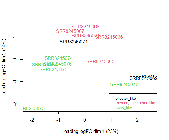
Visualizing your data with a Multidimensional scaling (MDS) plot.

plotMDS(d, col = as.numeric(factor(metadata$simplified_cell_type)), cex = 1)
legend("bottomright", text.col = 1:3, legend = levels(factor(metadata$simplified_cell_type)), cex = 0.8)

The MDS plot tells you A LOT about what to expect from your experiment.

3a. Extracting “normalized” expression table We use the cpm function with log=TRUE to obtain log-transformed normalized expression data. On the log scale, the data has less mean-dependent variability and is more suitable for plotting.

logcpm <- cpm(d, log=TRUE)
write.table(logcpm,"rnaseq_workshop_normalized_counts.txt",sep="\t",quote=F)

Quiz 2

4. Voom transformation and calculation of variance weights

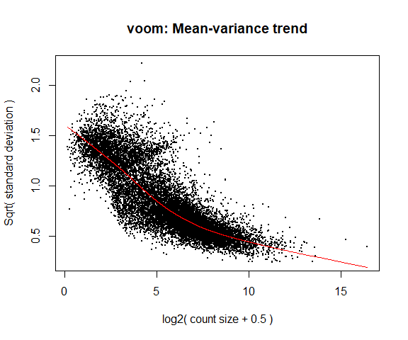
The voom is used to obtain variance weights for use in downstream statistical modelling, which assumes that the variability of a gene is independent of its expression.

4a. Voom

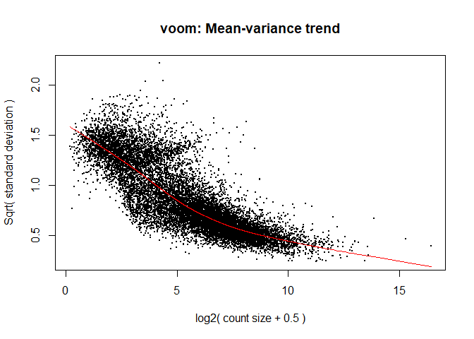
y <- voom(d, mm, plot = T)

What is voom doing?

Counts are transformed to log2 counts per million reads (CPM), where “per million reads” is defined based on the normalization factors we calculated earlier.
A linear model is fitted to the log2 CPM for each gene, and the residuals are calculated.
A smoothed curve is fitted to the sqrt(residual standard deviation) by average expression. (see red line in plot above)
The smoothed curve is used to obtain weights for each gene and sample that are passed into limma along with the log2 CPMs.

More details at “voom: precision weights unlock linear model analysis tools for RNA-seq read counts”

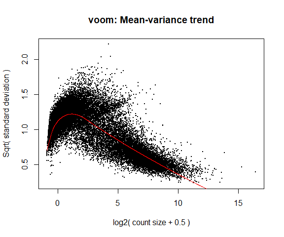
If your voom plot looks like the below (performed on the raw data), you might want to filter more:

tmp <- voom(d0, mm, plot = T)

5. Fitting linear models in limma

lmFit fits a linear model using weighted least squares for each gene:

fit <- lmFit(y, mm)
head(coef(fit))

simplified_cell_typeeffector_like ENSMUSG00000104017.2 1.0581142 ENSMUSG00000025900.14 0.8247494 ENSMUSG00000033845.14 5.9751519 ENSMUSG00000025903.15 6.4960704 ENSMUSG00000033813.16 5.5836994 ENSMUSG00000033793.13 6.7336026 simplified_cell_typememory_precursor_like ENSMUSG00000104017.2 1.366092 ENSMUSG00000025900.14 1.817405 ENSMUSG00000033845.14 6.123220 ENSMUSG00000025903.15 6.537393 ENSMUSG00000033813.16 5.543657 ENSMUSG00000033793.13 7.242839 simplified_cell_typenaive_like ENSMUSG00000104017.2 -0.8858157 ENSMUSG00000025900.14 -0.1645845 ENSMUSG00000033845.14 5.8741078 ENSMUSG00000025903.15 6.1799819 ENSMUSG00000033813.16 5.4037780 ENSMUSG00000033793.13 6.9410105

Comparisons between groups (log fold-changes) are obtained as contrasts of these fitted linear models.

6. Specify which groups to compare using contrasts:

Comparison between naive-like and memory precursor-like

contr <- makeContrasts(simplified_cell_typenaive_like - simplified_cell_typememory_precursor_like, levels = colnames(coef(fit)))

6a. Estimate contrast for each gene

tmp <- contrasts.fit(fit, contr)

Some genes may have particularly high or low variability even after transformation and weighting due to random variability, particularly with small sample sizes. Empirical Bayes smoothing of standard errors of log fold changes helps with this (shifts standard errors that are much larger or smaller than those from other genes towards the average standard error) (see “Linear Models and Empirical Bayes Methods for Assessing Differential Expression in Microarray Experiments”

6b. Apply EBayes

tmp <- eBayes(tmp)

7. Multiple Testing Adjustment

The topTable function reports sorted DE results and adjusts for multiple testing using method of Benjamini & Hochberg (BH), or its ‘alias’ fdr. “Controlling the false discovery rate: a practical and powerful approach to multiple testing.

here n=Inf says to produce the topTable for all genes.

top.table <- topTable(tmp, adjust.method = "BH", sort.by = "P", n = Inf)
head(top.table)

logFC AveExpr t P.Value adj.P.Val ENSMUSG00000000782.17 1.130285 9.058521 10.555268 1.124296e-08 8.804950e-05 ENSMUSG00000025017.11 -1.682138 7.213869 -10.284366 1.627415e-08 8.804950e-05 ENSMUSG00000045092.9 1.502989 8.309417 10.164093 1.922338e-08 8.804950e-05 ENSMUSG00000018899.18 1.145045 10.180757 9.810120 3.165608e-08 9.674879e-05 ENSMUSG00000042385.15 -3.575618 5.530089 -9.735911 3.520442e-08 9.674879e-05 ENSMUSG00000023132.9 -2.546520 7.426342 -9.286015 6.790147e-08 1.271304e-04 B ENSMUSG00000000782.17 10.227212 ENSMUSG00000025017.11 9.902773 ENSMUSG00000045092.9 9.758351 ENSMUSG00000018899.18 9.086943 ENSMUSG00000042385.15 8.242216 ENSMUSG00000023132.9 8.487412

Multiple Testing Correction

In ‘omics experiments, multiple testing correction is the standard in the field. Best choices are:

FDR (false discovery rate), such as Benjamini-Hochberg (1995).
Qvalue - Storey (2002)

The FDR-adjusted p-value (or qvalue) is a statement about the list and is no longer about the gene (pvalue). So a FDR of 0.05, says you expect 5% false positives among the list of genes with an FDR of 0.05 or less.

The statement “Statistically significantly different” means FDR of 0.05 or less.

7a. How many DE genes are there (false discovery rate corrected)?

length(which(top.table$adj.P.Val < 0.05))

[1] 791

8. Merge in annotation, check your results for confidence

You’ve conducted an experiment, you’ve seen a phenotype. Now check which genes are most differentially expressed (show the top 50)? Look up these top genes, their description and ensure they relate to your experiment/phenotype.

top.table$Gene.stable.ID <- sapply(strsplit(rownames(top.table), split = ".", fixed = TRUE), `[`, 1)
ord <- match(top.table$Gene.stable.ID, anno$Gene.stable.ID)
top.table$Gene.name <- anno$Gene.name[ord]
top.table$Gene.description <- anno$Gene.description[ord]
head(top.table, 50)

logFC AveExpr t P.Value adj.P.Val ENSMUSG00000000782.17 1.1302851 9.058521 10.555268 1.124296e-08 8.804950e-05 ENSMUSG00000025017.11 -1.6821378 7.213869 -10.284366 1.627415e-08 8.804950e-05 ENSMUSG00000045092.9 1.5029891 8.309417 10.164093 1.922338e-08 8.804950e-05 ENSMUSG00000018899.18 1.1450449 10.180757 9.810120 3.165608e-08 9.674879e-05 ENSMUSG00000042385.15 -3.5756182 5.530089 -9.735911 3.520442e-08 9.674879e-05 ENSMUSG00000023132.9 -2.5465202 7.426342 -9.286015 6.790147e-08 1.271304e-04 ENSMUSG00000039384.9 1.5770259 7.143061 9.253002 7.131760e-08 1.271304e-04 ENSMUSG00000020297.11 1.5685238 5.717637 9.228085 7.401524e-08 1.271304e-04 ENSMUSG00000029322.13 -0.9965664 8.530502 -8.928161 1.163675e-07 1.595087e-04 ENSMUSG00000079227.11 -1.8028257 7.363926 -8.889597 1.234318e-07 1.595087e-04 ENSMUSG00000091191.4 1.1655304 8.096354 8.867453 1.276905e-07 1.595087e-04 ENSMUSG00000034349.15 0.9635573 8.806433 8.802807 1.410287e-07 1.614897e-04 ENSMUSG00000075010.6 -0.9916741 9.340376 -8.568709 2.029396e-07 2.115879e-04 ENSMUSG00000028965.14 -3.4791121 6.870204 -8.530260 2.155761e-07 2.115879e-04 ENSMUSG00000053113.4 0.9340731 9.409133 8.483067 2.322238e-07 2.127325e-04 ENSMUSG00000040270.17 1.5841439 5.775190 8.439930 2.486223e-07 2.135199e-04 ENSMUSG00000030167.16 -1.8562225 7.625575 -8.283338 3.191151e-07 2.579389e-04 ENSMUSG00000018930.4 -2.1344241 7.532782 -8.237988 3.432334e-07 2.611590e-04 ENSMUSG00000006519.12 -0.9477292 7.960790 -8.186883 3.727180e-07 2.611590e-04 ENSMUSG00000030830.19 -0.9705894 9.576101 -8.170408 3.827791e-07 2.611590e-04 ENSMUSG00000020034.8 1.1967576 7.624316 8.144592 3.991223e-07 2.611590e-04 ENSMUSG00000050052.13 1.8442832 5.375312 8.115847 4.181825e-07 2.611930e-04 ENSMUSG00000015316.12 -2.0036280 6.464671 -8.075912 4.462601e-07 2.643524e-04 ENSMUSG00000027985.15 1.4793843 8.147842 8.038014 4.747355e-07 2.643524e-04 ENSMUSG00000021728.9 0.7288742 10.403827 8.014290 4.935249e-07 2.643524e-04 ENSMUSG00000112023.2 -1.4291587 9.056751 -7.969731 5.309510e-07 2.643524e-04 ENSMUSG00000112148.2 -1.7723555 6.655343 -7.962553 5.372527e-07 2.643524e-04 ENSMUSG00000021109.14 -0.8723171 8.468304 -7.960950 5.386701e-07 2.643524e-04 ENSMUSG00000017561.17 0.8127188 8.269992 7.771147 7.376954e-07 3.495404e-04 ENSMUSG00000020978.11 1.3479712 7.269913 7.709689 8.175741e-07 3.744762e-04 ENSMUSG00000049775.17 -0.8026414 9.941892 -7.575732 1.024685e-06 4.541997e-04 ENSMUSG00000026581.15 0.8419716 9.125156 7.530063 1.107278e-06 4.692204e-04 ENSMUSG00000030149.16 -1.4446697 8.593087 -7.519754 1.126867e-06 4.692204e-04 ENSMUSG00000029084.6 -1.5435018 5.647269 -7.479330 1.207245e-06 4.879046e-04 ENSMUSG00000015437.6 -2.8112472 9.468327 -7.439288 1.292793e-06 5.039672e-04 ENSMUSG00000037944.9 1.3602527 8.954916 7.426980 1.320342e-06 5.039672e-04 ENSMUSG00000004612.10 -0.7844487 9.918711 -7.198847 1.958934e-06 7.146273e-04 ENSMUSG00000022696.18 0.8821514 8.299524 7.193800 1.976263e-06 7.146273e-04 ENSMUSG00000005470.9 -2.0638904 4.505179 -7.144746 2.153258e-06 7.586645e-04 ENSMUSG00000025747.13 -1.7535015 4.808162 -7.074781 2.434843e-06 8.364296e-04 ENSMUSG00000002897.6 0.8709059 8.223009 7.055535 2.518859e-06 8.364890e-04 ENSMUSG00000024251.11 1.1074968 7.517188 7.034434 2.614455e-06 8.364890e-04 ENSMUSG00000038894.8 1.7338348 5.066124 7.033745 2.617643e-06 8.364890e-04 ENSMUSG00000020315.19 0.9573338 7.293769 7.009749 2.731119e-06 8.529160e-04 ENSMUSG00000066278.7 0.9187533 10.001012 6.877183 3.457565e-06 1.055787e-03 ENSMUSG00000018209.16 0.8270881 7.655715 6.857458 3.581790e-06 1.069943e-03 ENSMUSG00000049103.15 -1.8253828 6.871028 -6.844042 3.668933e-06 1.072656e-03 ENSMUSG00000075602.11 -1.5627410 8.403295 -6.784283 4.084807e-06 1.142292e-03 ENSMUSG00000055170.5 -2.2019101 5.076920 -6.782063 4.101173e-06 1.142292e-03 ENSMUSG00000020372.16 0.4616605 10.515691 6.774624 4.156509e-06 1.142292e-03 B Gene.stable.ID Gene.name ENSMUSG00000000782.17 10.227212 ENSMUSG00000000782 Tcf7 ENSMUSG00000025017.11 9.902773 ENSMUSG00000025017 Pik3ap1 ENSMUSG00000045092.9 9.758351 ENSMUSG00000045092 S1pr1 ENSMUSG00000018899.18 9.086943 ENSMUSG00000018899 Irf1 ENSMUSG00000042385.15 8.242216 ENSMUSG00000042385 Gzmk ENSMUSG00000023132.9 8.487412 ENSMUSG00000023132 Gzma ENSMUSG00000039384.9 8.481685 ENSMUSG00000039384 Dusp10 ENSMUSG00000020297.11 8.376917 ENSMUSG00000020297 Nsg2 ENSMUSG00000029322.13 7.908075 ENSMUSG00000029322 Plac8 ENSMUSG00000079227.11 7.945640 ENSMUSG00000079227 Ccr5 ENSMUSG00000091191.4 7.885146 ENSMUSG00000091191 Gm17334 ENSMUSG00000034349.15 7.698005 ENSMUSG00000034349 Smc4 ENSMUSG00000075010.6 7.277665 ENSMUSG00000075010 AW112010 ENSMUSG00000028965.14 7.356462 ENSMUSG00000028965 Tnfrsf9 ENSMUSG00000053113.4 7.134404 ENSMUSG00000053113 Socs3 ENSMUSG00000040270.17 7.177477 ENSMUSG00000040270 Bach2 ENSMUSG00000030167.16 7.005214 ENSMUSG00000030167 Klrc1 ENSMUSG00000018930.4 6.942369 ENSMUSG00000018930 Ccl4 ENSMUSG00000006519.12 6.818249 ENSMUSG00000006519 Cyba ENSMUSG00000030830.19 6.622206 ENSMUSG00000030830 Itgal ENSMUSG00000020034.8 6.771345 ENSMUSG00000020034 Tcp11l2 ENSMUSG00000050052.13 6.691590 ENSMUSG00000050052 Tdrp ENSMUSG00000015316.12 6.676951 ENSMUSG00000015316 Slamf1 ENSMUSG00000027985.15 6.559325 ENSMUSG00000027985 Lef1 ENSMUSG00000021728.9 6.186829 ENSMUSG00000021728 Emb ENSMUSG00000112023.2 6.360248 ENSMUSG00000112023 Lilrb4b ENSMUSG00000112148.2 6.510419 ENSMUSG00000112148 Lilrb4a ENSMUSG00000021109.14 6.390405 ENSMUSG00000021109 Hif1a ENSMUSG00000017561.17 6.098857 ENSMUSG00000017561 Crlf3 ENSMUSG00000020978.11 6.083307 ENSMUSG00000020978 Klhdc2 ENSMUSG00000049775.17 5.544348 ENSMUSG00000049775 Tmsb4x ENSMUSG00000026581.15 5.501182 ENSMUSG00000026581 Sell ENSMUSG00000030149.16 5.650246 ENSMUSG00000030149 Klrk1 ENSMUSG00000029084.6 5.680036 ENSMUSG00000029084 Cd38 ENSMUSG00000015437.6 5.457908 ENSMUSG00000015437 Gzmb ENSMUSG00000037944.9 5.354348 ENSMUSG00000037944 Ccr7 ENSMUSG00000004612.10 4.894014 ENSMUSG00000004612 Nkg7 ENSMUSG00000022696.18 5.086597 ENSMUSG00000022696 Sidt1 ENSMUSG00000005470.9 4.828071 ENSMUSG00000005470 Asf1b ENSMUSG00000025747.13 4.825342 ENSMUSG00000025747 Tyms ENSMUSG00000002897.6 4.880218 ENSMUSG00000002897 Il17ra ENSMUSG00000024251.11 4.884358 ENSMUSG00000024251 Thada ENSMUSG00000038894.8 4.917477 ENSMUSG00000038894 Irs2 ENSMUSG00000020315.19 4.883647 ENSMUSG00000020315 Sptbn1 ENSMUSG00000066278.7 4.295165 ENSMUSG00000066278 Vps37b ENSMUSG00000018209.16 4.582647 ENSMUSG00000018209 Stk4 ENSMUSG00000049103.15 4.635448 ENSMUSG00000049103 Ccr2 ENSMUSG00000075602.11 4.346635 ENSMUSG00000075602 Ly6a ENSMUSG00000055170.5 4.375381 ENSMUSG00000055170 Ifng ENSMUSG00000020372.16 3.983221 ENSMUSG00000020372 Rack1 Gene.description ENSMUSG00000000782.17 transcription factor 7, T cell specific [Source:MGI Symbol;Acc:MGI:98507] ENSMUSG00000025017.11 phosphoinositide-3-kinase adaptor protein 1 [Source:MGI Symbol;Acc:MGI:1933177] ENSMUSG00000045092.9 sphingosine-1-phosphate receptor 1 [Source:MGI Symbol;Acc:MGI:1096355] ENSMUSG00000018899.18 interferon regulatory factor 1 [Source:MGI Symbol;Acc:MGI:96590] ENSMUSG00000042385.15 granzyme K [Source:MGI Symbol;Acc:MGI:1298232] ENSMUSG00000023132.9 granzyme A [Source:MGI Symbol;Acc:MGI:109266] ENSMUSG00000039384.9 dual specificity phosphatase 10 [Source:MGI Symbol;Acc:MGI:1927070] ENSMUSG00000020297.11 neuron specific gene family member 2 [Source:MGI Symbol;Acc:MGI:1202070] ENSMUSG00000029322.13 placenta-specific 8 [Source:MGI Symbol;Acc:MGI:2445289] ENSMUSG00000079227.11 chemokine (C-C motif) receptor 5 [Source:MGI Symbol;Acc:MGI:107182] ENSMUSG00000091191.4 predicted gene, 17334 [Source:MGI Symbol;Acc:MGI:4936968] ENSMUSG00000034349.15 structural maintenance of chromosomes 4 [Source:MGI Symbol;Acc:MGI:1917349] ENSMUSG00000075010.6 expressed sequence AW112010 [Source:MGI Symbol;Acc:MGI:2147706] ENSMUSG00000028965.14 tumor necrosis factor receptor superfamily, member 9 [Source:MGI Symbol;Acc:MGI:1101059] ENSMUSG00000053113.4 suppressor of cytokine signaling 3 [Source:MGI Symbol;Acc:MGI:1201791] ENSMUSG00000040270.17 BTB and CNC homology, basic leucine zipper transcription factor 2 [Source:MGI Symbol;Acc:MGI:894679] ENSMUSG00000030167.16 killer cell lectin-like receptor subfamily C, member 1 [Source:MGI Symbol;Acc:MGI:1336161] ENSMUSG00000018930.4 chemokine (C-C motif) ligand 4 [Source:MGI Symbol;Acc:MGI:98261] ENSMUSG00000006519.12 cytochrome b-245, alpha polypeptide [Source:MGI Symbol;Acc:MGI:1316658] ENSMUSG00000030830.19 integrin alpha L [Source:MGI Symbol;Acc:MGI:96606] ENSMUSG00000020034.8 t-complex 11 (mouse) like 2 [Source:MGI Symbol;Acc:MGI:2444679] ENSMUSG00000050052.13 testis development related protein [Source:MGI Symbol;Acc:MGI:1919398] ENSMUSG00000015316.12 signaling lymphocytic activation molecule family member 1 [Source:MGI Symbol;Acc:MGI:1351314] ENSMUSG00000027985.15 lymphoid enhancer binding factor 1 [Source:MGI Symbol;Acc:MGI:96770] ENSMUSG00000021728.9 embigin [Source:MGI Symbol;Acc:MGI:95321] ENSMUSG00000112023.2 leukocyte immunoglobulin-like receptor, subfamily B, member 4B [Source:MGI Symbol;Acc:MGI:102702] ENSMUSG00000112148.2 leukocyte immunoglobulin-like receptor, subfamily B, member 4A [Source:MGI Symbol;Acc:MGI:102701] ENSMUSG00000021109.14 hypoxia inducible factor 1, alpha subunit [Source:MGI Symbol;Acc:MGI:106918] ENSMUSG00000017561.17 cytokine receptor-like factor 3 [Source:MGI Symbol;Acc:MGI:1860086] ENSMUSG00000020978.11 kelch domain containing 2 [Source:MGI Symbol;Acc:MGI:1916804] ENSMUSG00000049775.17 thymosin, beta 4, X chromosome [Source:MGI Symbol;Acc:MGI:99510] ENSMUSG00000026581.15 selectin, lymphocyte [Source:MGI Symbol;Acc:MGI:98279] ENSMUSG00000030149.16 killer cell lectin-like receptor subfamily K, member 1 [Source:MGI Symbol;Acc:MGI:1196250] ENSMUSG00000029084.6 CD38 antigen [Source:MGI Symbol;Acc:MGI:107474] ENSMUSG00000015437.6 granzyme B [Source:MGI Symbol;Acc:MGI:109267] ENSMUSG00000037944.9 chemokine (C-C motif) receptor 7 [Source:MGI Symbol;Acc:MGI:103011] ENSMUSG00000004612.10 natural killer cell group 7 sequence [Source:MGI Symbol;Acc:MGI:1931250] ENSMUSG00000022696.18 SID1 transmembrane family, member 1 [Source:MGI Symbol;Acc:MGI:2443155] ENSMUSG00000005470.9 anti-silencing function 1B histone chaperone [Source:MGI Symbol;Acc:MGI:1914179] ENSMUSG00000025747.13 thymidylate synthase [Source:MGI Symbol;Acc:MGI:98878] ENSMUSG00000002897.6 interleukin 17 receptor A [Source:MGI Symbol;Acc:MGI:107399] ENSMUSG00000024251.11 thyroid adenoma associated [Source:MGI Symbol;Acc:MGI:3039623] ENSMUSG00000038894.8 insulin receptor substrate 2 [Source:MGI Symbol;Acc:MGI:109334] ENSMUSG00000020315.19 spectrin beta, non-erythrocytic 1 [Source:MGI Symbol;Acc:MGI:98388] ENSMUSG00000066278.7 vacuolar protein sorting 37B [Source:MGI Symbol;Acc:MGI:1916724] ENSMUSG00000018209.16 serine/threonine kinase 4 [Source:MGI Symbol;Acc:MGI:1929004] ENSMUSG00000049103.15 chemokine (C-C motif) receptor 2 [Source:MGI Symbol;Acc:MGI:106185] ENSMUSG00000075602.11 lymphocyte antigen 6 complex, locus A [Source:MGI Symbol;Acc:MGI:107527] ENSMUSG00000055170.5 interferon gamma [Source:MGI Symbol;Acc:MGI:107656] ENSMUSG00000020372.16 receptor for activated C kinase 1 [Source:MGI Symbol;Acc:MGI:101849]

Columns are

logFC: log2 fold change of naive/memory
AveExpr: Average expression across all samples, in log2 CPM
t: logFC divided by its standard error
P.Value: Raw p-value (based on t) from test that logFC differs from 0
adj.P.Val: Benjamini-Hochberg false discovery rate adjusted p-value
B: log-odds that gene is DE (arguably less useful than the other columns)

9. Write top.table to a file

write.table(top.table, file = "naive_v_memory.txt", row.names = F, sep = "\t", quote = F)

Quiz 3

Linear models and contrasts

Let’s say we want to compare memory precursor-like to effector-like. The only thing we have to change is the call to makeContrasts:

contr <- makeContrasts(simplified_cell_typememory_precursor_like - simplified_cell_typeeffector_like, levels = colnames(coef(fit)))
tmp <- contrasts.fit(fit, contr)
tmp <- eBayes(tmp)
top.table <- topTable(tmp, sort.by = "P", n = Inf)
top.table$Gene.stable.ID <- sapply(strsplit(rownames(top.table), split = ".", fixed = TRUE), `[`, 1)
ord <- match(top.table$Gene.stable.ID, anno$Gene.stable.ID)
top.table$Gene.name <- anno$Gene.name[ord]
top.table$Gene.description <- anno$Gene.description[ord]
head(top.table, 20)

logFC AveExpr t P.Value adj.P.Val ENSMUSG00000023132.9 -2.5567801 7.426342 -14.004789 1.766660e-10 2.427567e-06 ENSMUSG00000026581.15 2.6301608 9.125156 12.022092 1.709164e-09 8.841501e-06 ENSMUSG00000052336.8 -4.5030532 2.925091 -11.922716 1.930318e-09 8.841501e-06 ENSMUSG00000030114.9 -3.6168624 2.619888 -10.857963 7.500415e-09 2.576580e-05 ENSMUSG00000029322.13 1.6331265 8.530502 10.555095 1.124560e-08 3.090515e-05 ENSMUSG00000035042.3 -1.2088127 10.526773 -10.175676 1.891628e-08 3.721173e-05 ENSMUSG00000022346.18 2.5599425 7.451979 10.174146 1.895656e-08 3.721173e-05 ENSMUSG00000022587.15 1.1072335 10.208831 9.627330 4.116897e-08 7.071285e-05 ENSMUSG00000102212.2 1.4951949 8.986555 8.981593 1.072737e-07 1.637831e-04 ENSMUSG00000000782.17 1.5619835 9.058521 8.818749 1.376090e-07 1.890885e-04 ENSMUSG00000076617.10 2.5055707 8.183406 8.666619 1.741457e-07 2.175396e-04 ENSMUSG00000037742.15 0.4777519 12.144310 8.561248 2.053294e-07 2.351193e-04 ENSMUSG00000032399.9 0.6405806 11.351774 8.497713 2.269177e-07 2.398520e-04 ENSMUSG00000067274.11 0.6500826 11.017720 8.292419 3.145028e-07 3.086845e-04 ENSMUSG00000032518.7 0.6125789 9.968261 8.213824 3.568571e-07 3.269049e-04 ENSMUSG00000025997.14 3.1386693 6.743643 7.938065 5.593465e-07 4.803737e-04 ENSMUSG00000031320.10 0.5559647 10.397342 7.855551 6.410677e-07 5.181712e-04 ENSMUSG00000031328.17 -1.1145751 8.758467 -7.803788 6.986342e-07 5.333296e-04 ENSMUSG00000030744.14 0.5433811 11.068420 7.727942 7.929471e-07 5.734677e-04 ENSMUSG00000024675.20 1.6668939 7.270476 7.483822 1.198025e-06 8.231032e-04 B Gene.stable.ID Gene.name ENSMUSG00000023132.9 14.310274 ENSMUSG00000023132 Gzma ENSMUSG00000026581.15 11.826636 ENSMUSG00000026581 Sell ENSMUSG00000052336.8 10.342165 ENSMUSG00000052336 Cx3cr1 ENSMUSG00000030114.9 9.030703 ENSMUSG00000030114 Klrg1 ENSMUSG00000029322.13 10.248833 ENSMUSG00000029322 Plac8 ENSMUSG00000035042.3 9.631361 ENSMUSG00000035042 Ccl5 ENSMUSG00000022346.18 9.241332 ENSMUSG00000022346 Myc ENSMUSG00000022587.15 8.975332 ENSMUSG00000022587 Ly6e ENSMUSG00000102212.2 8.077983 ENSMUSG00000102212 C230085N15Rik ENSMUSG00000000782.17 7.830467 ENSMUSG00000000782 Tcf7 ENSMUSG00000076617.10 7.517473 ENSMUSG00000076617 Ighm ENSMUSG00000037742.15 7.056406 ENSMUSG00000037742 Eef1a1 ENSMUSG00000032399.9 7.113131 ENSMUSG00000032399 Rpl4 ENSMUSG00000067274.11 6.827216 ENSMUSG00000067274 Rplp0 ENSMUSG00000032518.7 6.827883 ENSMUSG00000032518 Rpsa ENSMUSG00000025997.14 5.634781 ENSMUSG00000025997 Ikzf2 ENSMUSG00000031320.10 6.179851 ENSMUSG00000031320 Rps4x ENSMUSG00000031328.17 6.188865 ENSMUSG00000031328 Flna ENSMUSG00000030744.14 5.861835 ENSMUSG00000030744 Rps3 ENSMUSG00000024675.20 5.705245 ENSMUSG00000024675 Ms4a4c Gene.description ENSMUSG00000023132.9 granzyme A [Source:MGI Symbol;Acc:MGI:109266] ENSMUSG00000026581.15 selectin, lymphocyte [Source:MGI Symbol;Acc:MGI:98279] ENSMUSG00000052336.8 chemokine (C-X3-C motif) receptor 1 [Source:MGI Symbol;Acc:MGI:1333815] ENSMUSG00000030114.9 killer cell lectin-like receptor subfamily G, member 1 [Source:MGI Symbol;Acc:MGI:1355294] ENSMUSG00000029322.13 placenta-specific 8 [Source:MGI Symbol;Acc:MGI:2445289] ENSMUSG00000035042.3 chemokine (C-C motif) ligand 5 [Source:MGI Symbol;Acc:MGI:98262] ENSMUSG00000022346.18 myelocytomatosis oncogene [Source:MGI Symbol;Acc:MGI:97250] ENSMUSG00000022587.15 lymphocyte antigen 6 complex, locus E [Source:MGI Symbol;Acc:MGI:106651] ENSMUSG00000102212.2 RIKEN cDNA C230085N15 gene [Source:MGI Symbol;Acc:MGI:2444267] ENSMUSG00000000782.17 transcription factor 7, T cell specific [Source:MGI Symbol;Acc:MGI:98507] ENSMUSG00000076617.10 immunoglobulin heavy constant mu [Source:MGI Symbol;Acc:MGI:96448] ENSMUSG00000037742.15 eukaryotic translation elongation factor 1 alpha 1 [Source:MGI Symbol;Acc:MGI:1096881] ENSMUSG00000032399.9 ribosomal protein L4 [Source:MGI Symbol;Acc:MGI:1915141] ENSMUSG00000067274.11 ribosomal protein, large, P0 [Source:MGI Symbol;Acc:MGI:1927636] ENSMUSG00000032518.7 ribosomal protein SA [Source:MGI Symbol;Acc:MGI:105381] ENSMUSG00000025997.14 IKAROS family zinc finger 2 [Source:MGI Symbol;Acc:MGI:1342541] ENSMUSG00000031320.10 ribosomal protein S4, X-linked [Source:MGI Symbol;Acc:MGI:98158] ENSMUSG00000031328.17 filamin, alpha [Source:MGI Symbol;Acc:MGI:95556] ENSMUSG00000030744.14 ribosomal protein S3 [Source:MGI Symbol;Acc:MGI:1350917] ENSMUSG00000024675.20 membrane-spanning 4-domains, subfamily A, member 4C [Source:MGI Symbol;Acc:MGI:1927656]

A different way of fitting the same model

Above, we told R to fit a model using the formula ~0 + simplified_cell_type, which specifies a cell means model where each model coefficient is the mean of a group. However, by default R uses reference group parameterization, which corresponds to a model where the parameter called “(Intercept)” is a reference group and the other coefficients are the differences from that group.

These two models yield the same results in this case, so use whichever is most convenient.

mm <- model.matrix(~simplified_cell_type, data = metadata) # no 0 in front!
y <- voom(d, mm, plot = FALSE)
fit <- lmFit(y, mm)
head(coef(fit))

(Intercept) simplified_cell_typememory_precursor_like ENSMUSG00000104017.2 1.0581142 0.30797751 ENSMUSG00000025900.14 0.8247494 0.99265578 ENSMUSG00000033845.14 5.9751519 0.14806782 ENSMUSG00000025903.15 6.4960704 0.04132277 ENSMUSG00000033813.16 5.5836994 -0.04004208 ENSMUSG00000033793.13 6.7336026 0.50923595 simplified_cell_typenaive_like ENSMUSG00000104017.2 -1.9439299 ENSMUSG00000025900.14 -0.9893339 ENSMUSG00000033845.14 -0.1010441 ENSMUSG00000025903.15 -0.3160885 ENSMUSG00000033813.16 -0.1799214 ENSMUSG00000033793.13 0.2074080

Interpretation of model coefficients:

(Intercept) is the mean of the effector-like group
simplified_cell_typememory_precursor_like is the difference in means between memory precursor-like and effector-like
simplified_cell_typenaive_like is the difference in means between naive-like and effector-like.

(Effector-like is the refence group here because it’s first alphabetically.)

To compare memory precursor like to the following we test the simplified_cell_typememory_precursor_like coefficient, which is the second coefficient:

tmp <- contrasts.fit(fit, coef = 2) # test second coefficient
tmp <- eBayes(tmp)
top.table <- topTable(tmp, sort.by = "P", n = Inf)
top.table$Gene.stable.ID <- sapply(strsplit(rownames(top.table), split = ".", fixed = TRUE), `[`, 1)
ord <- match(top.table$Gene.stable.ID, anno$Gene.stable.ID)
top.table$Gene.name <- anno$Gene.name[ord]
top.table$Gene.description <- anno$Gene.description[ord]
head(top.table, 20)

Results are identical to what we obtained using the other parameterization.

More complicated models

Specifying a different model is simply a matter of changing the calls to model.matrix (and possibly to contrasts.fit).

What if we want to adjust for a continuous variable like the age of the mouse in weeks?

(We are making this data up here, but it would typically be a variable in your metadata.)

# Generate example age data
set.seed(99)
age <- sample(16:40, size = nrow(metadata), replace = TRUE)
age

[1] 31 16 27 37 37 36 18 25 17 21 28 35 19 19

metadata$age <- age

Model adjusting for age:

mm <- model.matrix(~0 + simplified_cell_type + age, data = metadata)
y <- voom(d, mm, plot = F)
fit <- lmFit(y, mm)
contr <- makeContrasts(simplified_cell_typenaive_like - simplified_cell_typememory_precursor_like,
  levels = colnames(coef(fit)))
tmp <- contrasts.fit(fit, contr)
tmp <- eBayes(tmp)
top.table <- topTable(tmp, sort.by = "P", n = Inf)
top.table$Gene.stable.ID <- sapply(strsplit(rownames(top.table), split = ".", fixed = TRUE), `[`, 1)
ord <- match(top.table$Gene.stable.ID, anno$Gene.stable.ID)
top.table$Gene.name <- anno$Gene.name[ord]
top.table$Gene.description <- anno$Gene.description[ord]
head(top.table, 20)

logFC AveExpr t P.Value adj.P.Val ENSMUSG00000042385.15 -3.464568 5.5300892 -14.099696 2.855095e-10 3.923186e-06 ENSMUSG00000023132.9 -2.486250 7.4263418 -12.232557 2.186596e-09 1.280022e-05 ENSMUSG00000006310.11 -5.623587 1.6953806 -12.022213 2.794604e-09 1.280022e-05 ENSMUSG00000067235.15 -3.780245 3.6661367 -11.284348 6.799676e-09 2.335859e-05 ENSMUSG00000040204.7 -7.052717 2.5371407 -10.216428 2.681798e-08 6.402620e-05 ENSMUSG00000031004.9 -4.562685 3.9421711 -10.185320 2.795701e-08 6.402620e-05 ENSMUSG00000025017.11 -1.610404 7.2138693 -9.874673 4.257998e-08 8.358449e-05 ENSMUSG00000114568.2 -5.668285 -0.4768492 -9.599167 6.235314e-08 8.640749e-05 ENSMUSG00000036223.17 -5.323309 1.1124639 -9.554962 6.633772e-08 8.640749e-05 ENSMUSG00000038252.14 -2.136129 5.3646435 -9.529117 6.879099e-08 8.640749e-05 ENSMUSG00000018899.18 1.200407 10.1807572 9.515519 7.012002e-08 8.640749e-05 ENSMUSG00000021965.4 -3.675883 1.9194618 -9.434011 7.867465e-08 8.640749e-05 ENSMUSG00000028832.12 -3.433937 3.0469290 -9.254709 1.016049e-07 8.640749e-05 ENSMUSG00000045092.9 1.527469 8.3094175 9.235089 1.045112e-07 8.640749e-05 ENSMUSG00000017716.16 -3.593796 3.5858761 -9.218516 1.070343e-07 8.640749e-05 ENSMUSG00000109394.3 -3.789365 1.6018850 -9.188231 1.118123e-07 8.640749e-05 ENSMUSG00000028965.14 -3.226446 6.8702039 -9.115778 1.241779e-07 8.640749e-05 ENSMUSG00000030167.16 -1.931980 7.6255753 -9.075055 1.317532e-07 8.640749e-05 ENSMUSG00000039396.12 -4.474681 1.8217047 -9.058737 1.349239e-07 8.640749e-05 ENSMUSG00000037313.17 -2.395992 4.3527792 -9.006744 1.455737e-07 8.640749e-05 B Gene.stable.ID Gene.name ENSMUSG00000042385.15 13.897654 ENSMUSG00000042385 Gzmk ENSMUSG00000023132.9 11.817922 ENSMUSG00000023132 Gzma ENSMUSG00000006310.11 9.505382 ENSMUSG00000006310 Zbtb32 ENSMUSG00000067235.15 10.495830 ENSMUSG00000067235 H2-Q10 ENSMUSG00000040204.7 7.898681 ENSMUSG00000040204 Pclaf ENSMUSG00000031004.9 9.308500 ENSMUSG00000031004 Mki67 ENSMUSG00000025017.11 8.855799 ENSMUSG00000025017 Pik3ap1 ENSMUSG00000114568.2 6.526672 ENSMUSG00000114568 Gm48732 ENSMUSG00000036223.17 7.083619 ENSMUSG00000036223 Ska1 ENSMUSG00000038252.14 8.525750 ENSMUSG00000038252 Ncapd2 ENSMUSG00000018899.18 7.965919 ENSMUSG00000018899 Irf1 ENSMUSG00000021965.4 7.747044 ENSMUSG00000021965 Ska3 ENSMUSG00000028832.12 7.971888 ENSMUSG00000028832 Stmn1 ENSMUSG00000045092.9 7.844084 ENSMUSG00000045092 S1pr1 ENSMUSG00000017716.16 8.017940 ENSMUSG00000017716 Birc5 ENSMUSG00000109394.3 7.215792 ENSMUSG00000109394 A230057D06Rik ENSMUSG00000028965.14 7.783384 ENSMUSG00000028965 Tnfrsf9 ENSMUSG00000030167.16 7.622831 ENSMUSG00000030167 Klrc1 ENSMUSG00000039396.12 7.053495 ENSMUSG00000039396 Neil3 ENSMUSG00000037313.17 7.807957 ENSMUSG00000037313 Tacc3 Gene.description ENSMUSG00000042385.15 granzyme K [Source:MGI Symbol;Acc:MGI:1298232] ENSMUSG00000023132.9 granzyme A [Source:MGI Symbol;Acc:MGI:109266] ENSMUSG00000006310.11 zinc finger and BTB domain containing 32 [Source:MGI Symbol;Acc:MGI:1891838] ENSMUSG00000067235.15 histocompatibility 2, Q region locus 10 [Source:MGI Symbol;Acc:MGI:95929] ENSMUSG00000040204.7 PCNA clamp associated factor [Source:MGI Symbol;Acc:MGI:1915276] ENSMUSG00000031004.9 antigen identified by monoclonal antibody Ki 67 [Source:MGI Symbol;Acc:MGI:106035] ENSMUSG00000025017.11 phosphoinositide-3-kinase adaptor protein 1 [Source:MGI Symbol;Acc:MGI:1933177] ENSMUSG00000114568.2 predicted gene, 48732 [Source:MGI Symbol;Acc:MGI:6098394] ENSMUSG00000036223.17 spindle and kinetochore associated complex subunit 1 [Source:MGI Symbol;Acc:MGI:1913718] ENSMUSG00000038252.14 non-SMC condensin I complex, subunit D2 [Source:MGI Symbol;Acc:MGI:1915548] ENSMUSG00000018899.18 interferon regulatory factor 1 [Source:MGI Symbol;Acc:MGI:96590] ENSMUSG00000021965.4 spindle and kinetochore associated complex subunit 3 [Source:MGI Symbol;Acc:MGI:3041235] ENSMUSG00000028832.12 stathmin 1 [Source:MGI Symbol;Acc:MGI:96739] ENSMUSG00000045092.9 sphingosine-1-phosphate receptor 1 [Source:MGI Symbol;Acc:MGI:1096355] ENSMUSG00000017716.16 baculoviral IAP repeat-containing 5 [Source:MGI Symbol;Acc:MGI:1203517] ENSMUSG00000109394.3 RIKEN cDNA A230057D06 gene [Source:MGI Symbol;Acc:MGI:2442922] ENSMUSG00000028965.14 tumor necrosis factor receptor superfamily, member 9 [Source:MGI Symbol;Acc:MGI:1101059] ENSMUSG00000030167.16 killer cell lectin-like receptor subfamily C, member 1 [Source:MGI Symbol;Acc:MGI:1336161] ENSMUSG00000039396.12 nei like 3 (E. coli) [Source:MGI Symbol;Acc:MGI:2384588] ENSMUSG00000037313.17 transforming, acidic coiled-coil containing protein 3 [Source:MGI Symbol;Acc:MGI:1341163]

length(which(top.table$adj.P.Val < 0.05))

[1] 1393

What if we want to look at the correlation of gene expression with a continuous variable like weight?

# Generate example mouse weight data
set.seed(99)
weight <- rnorm(n = nrow(metadata), mean = 22, sd = 3)
weight

[1] 22.64189 23.43897 22.26349 23.33158 20.91149 22.36802 19.40846 23.46887 [9] 20.90765 18.11727 19.76269 24.76465 24.25016 14.47434

metadata$weight <- weight

Specify model matrix:

mm <- model.matrix(~weight, data = metadata)
head(mm)

(Intercept) weight 1 1 22.64189 2 1 23.43897 3 1 22.26349 4 1 23.33158 5 1 20.91149 6 1 22.36802

y <- voom(d, mm, plot = F)
fit <- lmFit(y, mm)
tmp <- contrasts.fit(fit, coef = 2) # test "weight" coefficient
tmp <- eBayes(tmp)
top.table <- topTable(tmp, sort.by = "P", n = Inf)
head(top.table, 20)

logFC AveExpr t P.Value adj.P.Val ENSMUSG00000079018.11 -0.4792294 2.49975815 -6.160052 1.107803e-05 0.09543176 ENSMUSG00000022324.16 -0.5021422 2.11186961 -5.790928 2.281227e-05 0.09543176 ENSMUSG00000025582.5 -0.6596359 -0.09778388 -5.788868 2.290555e-05 0.09543176 ENSMUSG00000002289.17 -0.4205855 2.53000581 -5.642634 3.064677e-05 0.09543176 ENSMUSG00000037060.4 -0.5758086 1.94803150 -5.575587 3.505541e-05 0.09543176 ENSMUSG00000035385.6 -0.6290369 2.89633660 -5.489770 4.167022e-05 0.09543176 ENSMUSG00000027624.21 -0.4339349 0.88901085 -5.261658 6.626442e-05 0.13007706 ENSMUSG00000021822.4 -0.7202958 0.91021525 -4.989706 1.161181e-04 0.19944729 ENSMUSG00000034485.11 -0.6191968 -0.69034049 -4.855222 1.536967e-04 0.21248218 ENSMUSG00000020086.7 -0.5130054 -0.38427855 -4.852316 1.546337e-04 0.21248218 ENSMUSG00000024810.17 -0.6040569 0.74702316 -4.736107 1.973217e-04 0.24649062 ENSMUSG00000001870.17 -0.6940340 1.01671718 -4.677981 2.230174e-04 0.25107836 ENSMUSG00000062380.5 -0.4515725 1.33488915 -4.624046 2.499132e-04 0.25107836 ENSMUSG00000031750.16 -0.5378946 0.05431110 -4.613012 2.558109e-04 0.25107836 ENSMUSG00000056758.15 -0.4519997 2.05228428 -4.553654 2.900637e-04 0.26068915 ENSMUSG00000028776.15 -0.6086387 0.04875476 -4.505727 3.211077e-04 0.26068915 ENSMUSG00000029377.6 -0.7715592 -0.37251857 -4.467913 3.479738e-04 0.26068915 ENSMUSG00000026688.6 -0.3923141 2.29583203 -4.387404 4.130474e-04 0.26068915 ENSMUSG00000041548.5 -0.5523554 2.10231242 -4.374446 4.246221e-04 0.26068915 ENSMUSG00000058070.15 -0.5608496 0.56154540 -4.359938 4.379729e-04 0.26068915 B ENSMUSG00000079018.11 3.22122428 ENSMUSG00000022324.16 2.65385132 ENSMUSG00000025582.5 1.56599254 ENSMUSG00000002289.17 2.40817000 ENSMUSG00000037060.4 2.29157091 ENSMUSG00000035385.6 2.27988880 ENSMUSG00000027624.21 1.43942278 ENSMUSG00000021822.4 1.00435938 ENSMUSG00000034485.11 0.05151125 ENSMUSG00000020086.7 0.23031195 ENSMUSG00000024810.17 0.43899136 ENSMUSG00000001870.17 0.61153836 ENSMUSG00000062380.5 0.54785603 ENSMUSG00000031750.16 0.11550931 ENSMUSG00000056758.15 0.47888324 ENSMUSG00000028776.15 -0.01408685 ENSMUSG00000029377.6 -0.32991579 ENSMUSG00000026688.6 0.17118449 ENSMUSG00000041548.5 0.16447251 ENSMUSG00000058070.15 -0.14587861

length(which(top.table$adj.P.Val < 0.05))

[1] 0

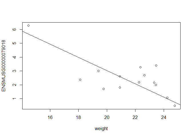
In this case, limma is fitting a linear regression model, which here is a straight line fit, with the slope and intercept defined by the model coefficients:

ENSMUSG00000079018 <- y$E["ENSMUSG00000079018.11",]
plot(ENSMUSG00000079018 ~ weight)
intercept <- coef(fit)["ENSMUSG00000079018.11", "(Intercept)"]
slope <- coef(fit)["ENSMUSG00000079018.11", "weight"]
abline(a = intercept, b = slope)

slope

[1] -0.4792294

In this example, the log fold change logFC is the slope of the line, or the change in gene expression (on the log2 CPM scale) for each unit increase in weight.

Here, a logFC of -0.47 means a 0.47 log2 CPM decrease in gene expression for each unit increase in weight, or a 39% decrease on the CPM scale (2^-0.47 = 0.717).

A bit more on linear models

Limma fits a linear model to each gene.

Linear models include analysis of variance (ANOVA) models, linear regression, and any model of the form

Y = β₀ + β₁X₁ + β₂X₂ + … + β_pX_p + ε

The covariates X can be:

a continuous variable (age, weight, temperature, etc.)
Dummy variables coding a categorical covariate (like cell type, genotype, and group)

The β’s are unknown parameters to be estimated.

In limma, the β’s are the log fold changes.

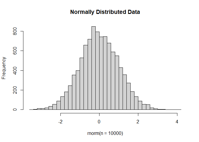
The error (residual) term ε is assumed to be normally distributed with a variance that is constant across the range of the data.

Normally distributed means the residuals come from a distribution that looks like this:

The log2 transformation that voom applies to the counts makes the data “normal enough”, but doesn’t completely stabilize the variance:

mm <- model.matrix(~0 + simplified_cell_type, data = metadata)
tmp <- voom(d, mm, plot = T)

The log2 counts per million are more variable at lower expression levels. The variance weights calculated by voom address this situation.

Both edgeR and limma have VERY comprehensive user manuals

The limma users’ guide has great details on model specification.

Quiz 4

Simple plotting

mm <- model.matrix(~0 + simplified_cell_type, data = metadata)
y <- voom(d, mm, plot = F)
fit <- lmFit(y, mm)
contrast.matrix <- makeContrasts(simplified_cell_typenaive_like - simplified_cell_typememory_precursor_like, levels=colnames(coef(fit)))
fit2 <- contrasts.fit(fit, contrast.matrix)
fit2 <- eBayes(fit2)
top.table <- topTable(fit2, n = 20)
top.table$Gene.stable.ID <- sapply(strsplit(rownames(top.table), split = ".", fixed = TRUE), `[`, 1)
ord <- match(top.table$Gene.stable.ID, anno$Gene.stable.ID)
top.table$Gene.name <- anno$Gene.name[ord]

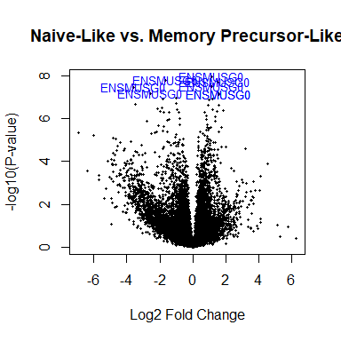
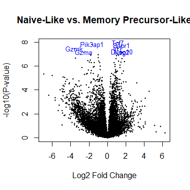
Volcano plot

# A version that needs some finessing
volcanoplot(fit2, highlight=8, names=rownames(fit2), main="Naive-Like vs. Memory Precursor-Like")

# A better version
volcanoplot(fit2, highlight=8, names=anno[match(sapply(strsplit(rownames(fit2), split = ".", fixed = TRUE), `[`, 1), anno$Gene.stable.ID), "Gene.name"], main="Naive-Like vs. Memory Precursor-Like")

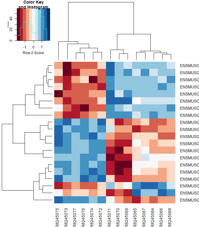
Heatmap

#using a red and blue color scheme without traces and scaling each row
heatmap.2(logcpm[rownames(top.table),],col=brewer.pal(11,"RdBu"),scale="row", trace="none")

# With gene names
heatmap.2(logcpm[rownames(top.table),],col=brewer.pal(11,"RdBu"),scale="row", trace="none", labRow = top.table$Gene.name)

sessionInfo()

R version 4.1.3 (2022-03-10) Platform: x86_64-w64-mingw32/x64 (64-bit) Running under: Windows 10 x64 (build 19044) Matrix products: default locale: [1] LC_COLLATE=English_United States.1252 [2] LC_CTYPE=English_United States.1252 [3] LC_MONETARY=English_United States.1252 [4] LC_NUMERIC=C [5] LC_TIME=English_United States.1252 attached base packages: [1] stats graphics grDevices datasets utils methods base other attached packages: [1] gplots_3.1.1 RColorBrewer_1.1-3 edgeR_3.36.0 limma_3.50.3 loaded via a namespace (and not attached): [1] Rcpp_1.0.8.3 knitr_1.38 magrittr_2.0.3 lattice_0.20-45 [5] R6_2.5.1 rlang_1.0.2 fastmap_1.1.0 highr_0.9 [9] stringr_1.4.0 caTools_1.18.2 tools_4.1.3 grid_4.1.3 [13] xfun_0.30 KernSmooth_2.23-20 cli_3.2.0 jquerylib_0.1.4 [17] gtools_3.9.2 htmltools_0.5.2 yaml_2.3.5 digest_0.6.29 [21] bitops_1.0-7 sass_0.4.1 evaluate_0.15 rmarkdown_2.13 [25] stringi_1.7.6 compiler_4.1.3 bslib_0.3.1 locfit_1.5-9.5 [29] jsonlite_1.8.0 renv_0.15.4

☰ Menu

RNA Seq Differential Expression and Enrichment Analysis