☰ Menu

      RNA Seq Differential Expression and Enrichment Analysis

Home
Preliminaries
Before the course
File downloads
Data Analysis
Differential Expression
Enrichment Analysis
R Code for Quizzes
Upcoming
Upcoming Bioinformatics Core Courses

GO AND KEGG Enrichment Analysis

Load libraries

suppressPackageStartupMessages(library(topGO))
suppressPackageStartupMessages(library(KEGGREST))
suppressPackageStartupMessages(library(org.Mm.eg.db))
suppressPackageStartupMessages(library(pathview))

If you did not create the file naive_v_memory.txt as part of the DE analysis, you can download it by running this code:

download.file("https://raw.githubusercontent.com/ucdavis-bioinformatics-training/2022-April-GGI-DE-in-R/master/data_analysis/naive_v_memory.txt", file.path(getwd(), "naive_v_memory.txt"))

Gene Ontology (GO) Enrichment

Gene ontology provides a controlled vocabulary for describing biological processes (BP ontology), molecular functions (MF ontology) and cellular components (CC ontology)

The GO ontologies themselves are organism-independent; terms are associated with genes for a specific organism through direct experimentation or through sequence homology with another organism and its GO annotation.

Terms are related to other terms through parent-child relationships in a directed acylic graph.

Enrichment analysis provides one way of drawing conclusions about a set of differential expression results.

1. topGO Example Using Kolmogorov-Smirnov Testing Our first example uses Kolmogorov-Smirnov Testing for enrichment testing of our mouse DE results, with GO annotation obtained from the Bioconductor database org.Mm.eg.db.

The first step in each topGO analysis is to create a topGOdata object. This contains the genes, the score for each gene (here we use the p-value from the DE test), the GO terms associated with each gene, and the ontology to be used (here we use the biological process ontology)

infile <- "naive_v_memory.txt"
tmp <- read.delim(infile)

geneList <- tmp$P.Value
xx <- as.list(org.Mm.egENSEMBL2EG)
names(geneList) <- xx[tmp$Gene.stable.ID] # Convert to entrezgene IDs
head(geneList)
21414 83490 13609 16362 14945 14938 1.124296e-08 1.627415e-08 1.922338e-08 3.165608e-08 3.520442e-08 6.790147e-08
# Create topGOData object
GOdata <- new("topGOdata",
	ontology = "BP",
	allGenes = geneList,
	geneSelectionFun = function(x)x,
	annot = annFUN.org , mapping = "org.Mm.eg.db")
Building most specific GOs .....
( 10766 GO terms found. )
Build GO DAG topology ..........
( 14415 GO terms and 32761 relations. )
Annotating nodes ...............
( 11359 genes annotated to the GO terms. )

2. The topGOdata object is then used as input for enrichment testing:

# Kolmogorov-Smirnov testing
resultKS <- runTest(GOdata, algorithm = "weight01", statistic = "ks")
-- Weight01 Algorithm -- the algorithm is scoring 14415 nontrivial nodes parameters: test statistic: ks score order: increasing
Level 20: 1 nodes to be scored (0 eliminated genes)
Level 19: 9 nodes to be scored (0 eliminated genes)
Level 18: 21 nodes to be scored (2 eliminated genes)
Level 17: 42 nodes to be scored (29 eliminated genes)
Level 16: 92 nodes to be scored (65 eliminated genes)
Level 15: 192 nodes to be scored (138 eliminated genes)
Level 14: 368 nodes to be scored (370 eliminated genes)
Level 13: 672 nodes to be scored (814 eliminated genes)
Level 12: 1153 nodes to be scored (1756 eliminated genes)
Level 11: 1627 nodes to be scored (3407 eliminated genes)
Level 10: 2063 nodes to be scored (5021 eliminated genes)
Level 9: 2165 nodes to be scored (6283 eliminated genes)
Level 8: 1957 nodes to be scored (7514 eliminated genes)
Level 7: 1670 nodes to be scored (8480 eliminated genes)
Level 6: 1221 nodes to be scored (9192 eliminated genes)
Level 5: 683 nodes to be scored (9671 eliminated genes)
Level 4: 327 nodes to be scored (9968 eliminated genes)
Level 3: 127 nodes to be scored (10097 eliminated genes)
Level 2: 24 nodes to be scored (10157 eliminated genes)
Level 1: 1 nodes to be scored (10205 eliminated genes)
tab <- GenTable(GOdata, raw.p.value = resultKS, topNodes = length(resultKS@score), numChar = 120)

topGO by default preferentially tests more specific terms, utilizing the topology of the GO graph. The algorithms used are described in detail here.

head(tab, 15)
GO.ID 1 GO:0007052 2 GO:0007608 3 GO:0035556 4 GO:0018105 5 GO:0010498 6 GO:0051382 7 GO:0007623 8 GO:0042776 9 GO:0010592 10 GO:0007186 11 GO:0000070 12 GO:0035278 13 GO:0051301 14 GO:0090050 15 GO:0046827 Term 1 mitotic spindle organization 2 sensory perception of smell 3 intracellular signal transduction 4 peptidyl-serine phosphorylation 5 proteasomal protein catabolic process 6 kinetochore assembly 7 circadian rhythm 8 mitochondrial ATP synthesis coupled proton transport 9 positive regulation of lamellipodium assembly 10 G protein-coupled receptor signaling pathway 11 mitotic sister chromatid segregation 12 miRNA mediated inhibition of translation 13 cell division 14 positive regulation of cell migration involved in sprouting angiogenesis 15 positive regulation of protein export from nucleus Annotated Significant Expected raw.p.value 1 103 103 103 2.5e-05 2 75 75 75 3.4e-05 3 1763 1763 1763 9.9e-05 4 239 239 239 0.00010 5 428 428 428 0.00012 6 17 17 17 0.00025 7 140 140 140 0.00029 8 15 15 15 0.00034 9 23 23 23 0.00035 10 362 362 362 0.00048 11 142 142 142 0.00065 12 14 14 14 0.00065 13 484 484 484 0.00067 14 15 15 15 0.00088 15 18 18 18 0.00096

The Kolmogorov-Smirnov test directly compares two probability distributions based on their maximum distance.

To illustrate the KS test, we plot probability distributions of p-values that are and that are not annotated with the term GO:0048699 “generation of neurons” (1008 genes)m p-value 1.000. (This won’t exactly match what topGO does due to their elimination algorithm):

rna.pp.terms <- genesInTerm(GOdata)[["GO:0048699"]] # get genes associated with term
p.values.in <- geneList[names(geneList) %in% rna.pp.terms]
p.values.out <- geneList[!(names(geneList) %in% rna.pp.terms)]
plot.ecdf(p.values.in, verticals = T, do.points = F, col = "red", lwd = 2, xlim = c(0,1),
          main = "Empirical Distribution of DE P-Values by Annotation with 'generation of neurons'",
          cex.main = 0.9, xlab = "p", ylab = "Probabilty(P-Value < p)")
ecdf.out <- ecdf(p.values.out)
xx <- unique(sort(c(seq(0, 1, length = 201), knots(ecdf.out))))
lines(xx, ecdf.out(xx), col = "black", lwd = 2)
legend("bottomright", legend = c("Genes Annotated with 'generation of neurons'", "Other genes'"), lwd = 2, col = 2:1, cex = 0.9)

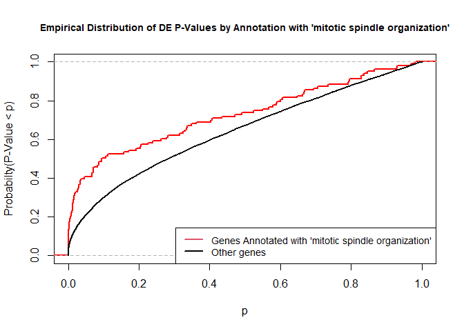
versus the probability distributions of p-values that are and that are not annotated with the term GO:0007052 “mitotic spindle organization” (103 genes) p-value 2.5x10⁻⁵.

rna.pp.terms <- genesInTerm(GOdata)[["GO:0007052"]] # get genes associated with term
p.values.in <- geneList[names(geneList) %in% rna.pp.terms]
p.values.out <- geneList[!(names(geneList) %in% rna.pp.terms)]
plot.ecdf(p.values.in, verticals = T, do.points = F, col = "red", lwd = 2, xlim = c(0,1),
          main = "Empirical Distribution of DE P-Values by Annotation with 'mitotic spindle organization'",
          cex.main = 0.9, xlab = "p", ylab = "Probabilty(P-Value < p)")
ecdf.out <- ecdf(p.values.out)
xx <- unique(sort(c(seq(0, 1, length = 201), knots(ecdf.out))))
lines(xx, ecdf.out(xx), col = "black", lwd = 2)
legend("bottomright", legend = c("Genes Annotated with 'mitotic spindle organization'", "Other genes"), lwd = 2, col = 2:1, cex = 0.9)

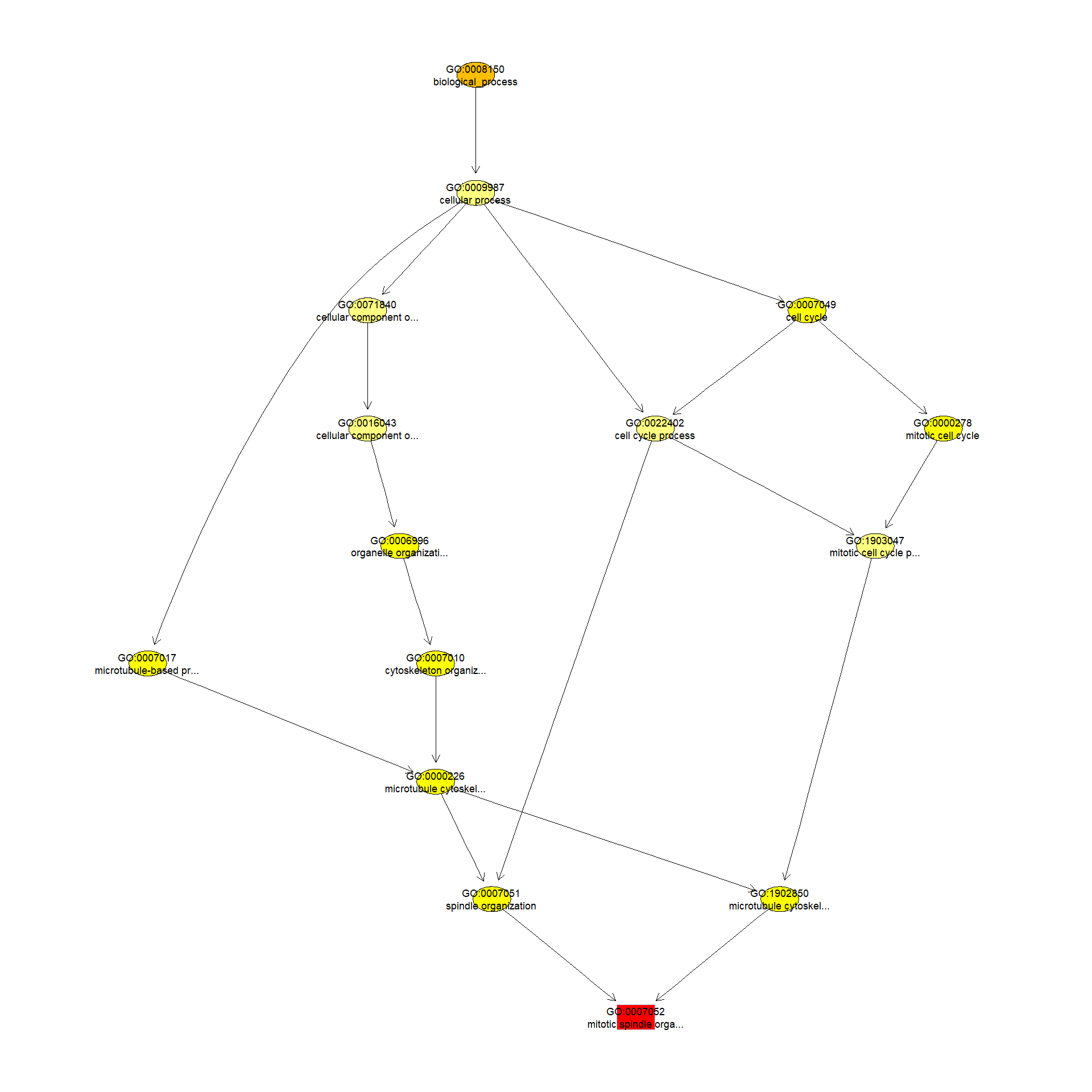
We can use the function showSigOfNodes to plot the GO graph for the most significant term and its parents, color coded by enrichment p-value (red is most significant):

par(cex = 0.3)
showSigOfNodes(GOdata, score(resultKS), firstSigNodes = 1, useInfo = "def")

$dag A graphNEL graph with directed edges Number of Nodes = 15 Number of Edges = 20 $complete.dag [1] "A graph with 15 nodes."
par(cex = 1)

3. topGO Example Using Fisher’s Exact Test

Next, we use Fisher’s exact test to test for GO enrichment among significantly DE genes.

Create topGOdata object:

# Create topGOData object
GOdata <- new("topGOdata",
	ontology = "BP",
	allGenes = geneList,
	geneSelectionFun = function(x) (x < 0.05),
	annot = annFUN.org , mapping = "org.Mm.eg.db")
Building most specific GOs .....
( 10766 GO terms found. )
Build GO DAG topology ..........
( 14415 GO terms and 32761 relations. )
Annotating nodes ...............
( 11359 genes annotated to the GO terms. )

Run Fisher’s Exact Test:

resultFisher <- runTest(GOdata, algorithm = "elim", statistic = "fisher")
-- Elim Algorithm -- the algorithm is scoring 10040 nontrivial nodes parameters: test statistic: fisher cutOff: 0.01
Level 20: 1 nodes to be scored (0 eliminated genes)
Level 19: 8 nodes to be scored (0 eliminated genes)
Level 18: 13 nodes to be scored (0 eliminated genes)
Level 17: 24 nodes to be scored (15 eliminated genes)
Level 16: 58 nodes to be scored (15 eliminated genes)
Level 15: 129 nodes to be scored (22 eliminated genes)
Level 14: 226 nodes to be scored (57 eliminated genes)
Level 13: 389 nodes to be scored (217 eliminated genes)
Level 12: 664 nodes to be scored (1229 eliminated genes)
Level 11: 1007 nodes to be scored (1448 eliminated genes)
Level 10: 1358 nodes to be scored (1759 eliminated genes)
Level 9: 1517 nodes to be scored (2091 eliminated genes)
Level 8: 1421 nodes to be scored (2862 eliminated genes)
Level 7: 1269 nodes to be scored (3412 eliminated genes)
Level 6: 966 nodes to be scored (3787 eliminated genes)
Level 5: 569 nodes to be scored (4752 eliminated genes)
Level 4: 279 nodes to be scored (5561 eliminated genes)
Level 3: 118 nodes to be scored (5696 eliminated genes)
Level 2: 23 nodes to be scored (6363 eliminated genes)
Level 1: 1 nodes to be scored (6363 eliminated genes)
tab <- GenTable(GOdata, raw.p.value = resultFisher, topNodes = length(resultFisher@score),
				numChar = 120)
head(tab)
GO.ID Term Annotated Significant 1 GO:0032465 regulation of cytokinesis 67 32 2 GO:0007052 mitotic spindle organization 103 42 3 GO:0007186 G protein-coupled receptor signaling pathway 362 113 4 GO:0007608 sensory perception of smell 75 32 5 GO:0051016 barbed-end actin filament capping 21 13 6 GO:1902969 mitotic DNA replication 14 10 Expected raw.p.value 1 14.97 3.8e-06 2 23.01 1.9e-05 3 80.87 4.5e-05 4 16.75 6.5e-05 5 4.69 0.00011 6 3.13 0.00012

Fisher’s Exact Test is applied to the table:

Significance/Annotation Annotated With GO Term Not Annotated With GO Term
Significantly DE n1 n3
Not Significantly DE n2 n4

and compares the probability of the observed table, conditional on the row and column sums, to what would be expected under random chance.

Advantages over KS (or Wilcoxon) Tests:

Disadvantages:

Quiz 1

##. KEGG Pathway Enrichment Testing With KEGGREST 
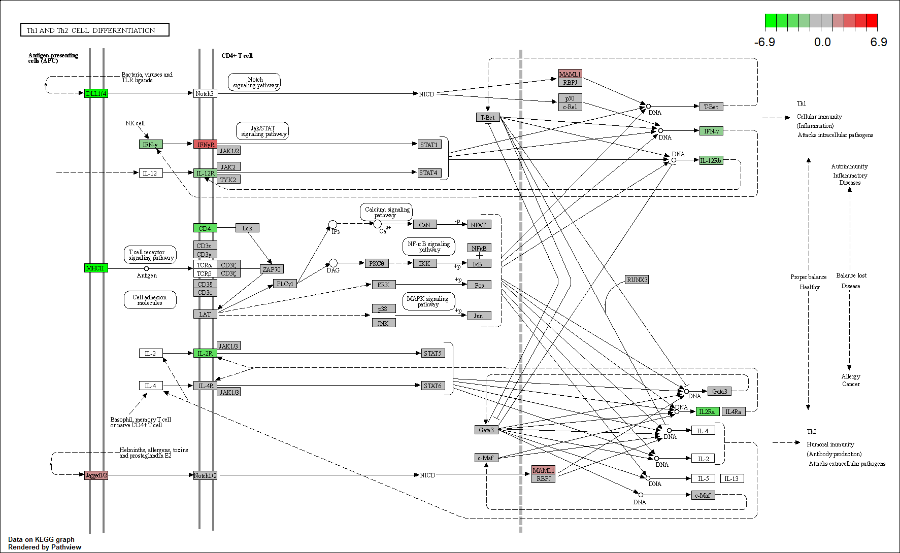
KEGG, the Kyoto Encyclopedia of Genes and Genomes (https://www.genome.jp/kegg/), provides assignment of genes for many organisms into pathways.

We will access KEGG pathway assignments for mouse through the KEGGREST Bioconductor package, and then use some homebrew code for enrichment testing.

1. Get all mouse pathways and their genes:

# Pull all pathways for mmu
pathways.list <- keggList("pathway", "mmu")
head(pathways.list)
path:mmu00010 "Glycolysis / Gluconeogenesis - Mus musculus (mouse)" path:mmu00020 "Citrate cycle (TCA cycle) - Mus musculus (mouse)" path:mmu00030 "Pentose phosphate pathway - Mus musculus (mouse)" path:mmu00040 "Pentose and glucuronate interconversions - Mus musculus (mouse)" path:mmu00051 "Fructose and mannose metabolism - Mus musculus (mouse)" path:mmu00052 "Galactose metabolism - Mus musculus (mouse)"
# Pull all genes for each pathway
pathway.codes <- sub("path:", "", names(pathways.list))
genes.by.pathway <- sapply(pathway.codes,
	function(pwid){
		pw <- keggGet(pwid)
		if (is.null(pw[[1]]$GENE)) return(NA)
		pw2 <- pw[[1]]$GENE[c(TRUE,FALSE)] 
		pw2 <- unlist(lapply(strsplit(pw2, split = ";", fixed = T), function(x)x[1]))
		return(pw2)
	}
)
head(genes.by.pathway)
$mmu00010 [1] "15277" "212032" "15275" "216019" "103988" "14751" [7] "18641" "18642" "56421" "14121" "14120" "11674" [13] "230163" "11676" "353204" "79459" "21991" "14433" [19] "115487111" "14447" "18655" "18663" "18648" "56012" [25] "13806" "13807" "13808" "433182" "226265" "18746" [31] "18770" "18597" "18598" "68263" "235339" "13382" [37] "16828" "16832" "16833" "106557" "11522" "11529" [43] "26876" "11532" "58810" "11669" "11671" "72535" [49] "110695" "56752" "11670" "67689" "621603" "73458" [55] "68738" "60525" "319625" "72157" "66681" "14377" [61] "14378" "68401" "72141" "12183" "17330" "18534" [67] "74551" $mmu00020 [1] "12974" "71832" "104112" "11429" "11428" "15926" "269951" "15929" [9] "67834" "170718" "243996" "18293" "239017" "78920" "13382" "56451" [17] "20917" "20916" "66945" "67680" "66052" "66925" "14194" "17449" [25] "17448" "18563" "18534" "74551" "18597" "18598" "68263" "235339" $mmu00030 [1] "14751" "14380" "14381" "66171" "100198" "110208" "66646" "21881" [9] "83553" "74419" "21351" "19895" "232449" "71336" "72157" "66681" [17] "19139" "110639" "328099" "75456" "19733" "75731" "235582" "11674" [25] "230163" "11676" "353204" "79459" "14121" "14120" "18641" "18642" [33] "56421" $mmu00040 [1] "110006" "16591" "22238" "22236" "94284" "94215" "394434" "394430" [9] "394432" "394433" "72094" "552899" "71773" "394435" "394436" "100727" [17] "231396" "100559" "112417" "243085" "613123" "22235" "216558" "58810" [25] "68631" "66646" "102448" "11997" "14187" "11677" "67861" "67880" [33] "20322" "71755" "75847" $mmu00051 [1] "110119" "54128" "29858" "331026" "69080" "218138" "22122" "75540" [9] "234730" "15277" "212032" "15275" "216019" "18641" "18642" "56421" [17] "14121" "14120" "18639" "18640" "170768" "270198" "319801" "16548" [25] "20322" "11997" "14187" "11677" "67861" "11674" "230163" "11676" [33] "353204" "79459" "21991" "225913" $mmu00052 [1] "319625" "14635" "14430" "74246" "216558" "72157" "66681" "15277" [9] "212032" "15275" "216019" "103988" "14377" "14378" "68401" "12091" [17] "226413" "16770" "14595" "53418" "11605" "11997" "14187" "11677" [25] "67861" "18641" "18642" "56421" "232714" "14387" "76051" "69983"

Read in DE file to be used in enrichment testing:

head(geneList)
21414 83490 13609 16362 14945 14938 1.124296e-08 1.627415e-08 1.922338e-08 3.165608e-08 3.520442e-08 6.790147e-08

2. Apply Wilcoxon rank-sum test to each pathway, testing if “in” p-values are smaller than “out” p-values:

# Wilcoxon test for each pathway
pVals.by.pathway <- t(sapply(names(genes.by.pathway),
	function(pathway) {
		pathway.genes <- genes.by.pathway[[pathway]]
		list.genes.in.pathway <- intersect(names(geneList), pathway.genes)
		list.genes.not.in.pathway <- setdiff(names(geneList), list.genes.in.pathway)
		scores.in.pathway <- geneList[list.genes.in.pathway]
		scores.not.in.pathway <- geneList[list.genes.not.in.pathway]
		if (length(scores.in.pathway) > 0){
			p.value <- wilcox.test(scores.in.pathway, scores.not.in.pathway, alternative = "less")$p.value
		} else{
			p.value <- NA
		}
		return(c(p.value = p.value, Annotated = length(list.genes.in.pathway)))
	}
))

# Assemble output table
outdat <- data.frame(pathway.code = rownames(pVals.by.pathway))
outdat$pathway.name <- pathways.list[paste0("path:",outdat$pathway.code)]
outdat$p.value <- pVals.by.pathway[,"p.value"]
outdat$Annotated <- pVals.by.pathway[,"Annotated"]
outdat <- outdat[order(outdat$p.value),]
head(outdat, 15)
pathway.code 215 mmu04740 340 mmu05415 269 mmu05020 264 mmu05010 242 mmu04932 341 mmu05416 334 mmu05330 301 mmu05200 193 mmu04658 335 mmu05332 330 mmu05320 174 mmu04514 331 mmu05321 106 mmu03030 270 mmu05022 pathway.name 215 Olfactory transduction - Mus musculus (mouse) 340 Diabetic cardiomyopathy - Mus musculus (mouse) 269 Prion disease - Mus musculus (mouse) 264 Alzheimer disease - Mus musculus (mouse) 242 Non-alcoholic fatty liver disease - Mus musculus (mouse) 341 Viral myocarditis - Mus musculus (mouse) 334 Allograft rejection - Mus musculus (mouse) 301 Pathways in cancer - Mus musculus (mouse) 193 Th1 and Th2 cell differentiation - Mus musculus (mouse) 335 Graft-versus-host disease - Mus musculus (mouse) 330 Autoimmune thyroid disease - Mus musculus (mouse) 174 Cell adhesion molecules - Mus musculus (mouse) 331 Inflammatory bowel disease - Mus musculus (mouse) 106 DNA replication - Mus musculus (mouse) 270 Pathways of neurodegeneration - multiple diseases - Mus musculus (mouse) p.value Annotated 215 2.214277e-06 88 340 2.260240e-06 160 269 3.147476e-06 216 264 1.129108e-05 292 242 1.223252e-05 124 341 2.009046e-05 50 334 2.762872e-05 29 301 3.440934e-05 356 193 4.016787e-05 74 335 5.295053e-05 30 330 8.420246e-05 29 174 9.039036e-05 82 331 1.542396e-04 40 106 1.716499e-04 35 270 2.982266e-04 355

The Wilcoxon rank-sum test is the nonparametric analogue of the two-sample t-test. It compares the ranks of observations in two groups. It is more powerful than the Kolmogorov-Smirnov test for location tests.

2. Plotting Pathways

foldChangeList <- tmp$logFC
xx <- as.list(org.Mm.egENSEMBL2EG)
names(foldChangeList) <- xx[tmp$Gene.stable.ID]
head(foldChangeList)
21414 83490 13609 16362 14945 14938 1.130285 -1.682138 1.502989 1.145045 -3.575618 -2.546520
mmu04658 <- pathview(gene.data  = foldChangeList,
                     pathway.id = "mmu04658",
                     species    = "mmu",
                     limit      = list(gene=max(abs(foldChangeList)), cpd=1))
'select()' returned 1:1 mapping between keys and columns
Info: Working in directory C:/Users/bpdurbin/Desktop/GGI_DE_course
Info: Writing image file mmu04658.pathview.png
Info: some node width is different from others, and hence adjusted!

Quiz 2

sessionInfo()
R version 4.1.3 (2022-03-10) Platform: x86_64-w64-mingw32/x64 (64-bit) Running under: Windows 10 x64 (build 19044) Matrix products: default locale: [1] LC_COLLATE=English_United States.1252 [2] LC_CTYPE=English_United States.1252 [3] LC_MONETARY=English_United States.1252 [4] LC_NUMERIC=C [5] LC_TIME=English_United States.1252 attached base packages: [1] grid stats4 stats graphics grDevices datasets utils [8] methods base other attached packages: [1] Rgraphviz_2.38.0 pathview_1.34.0 org.Mm.eg.db_3.14.0 [4] KEGGREST_1.34.0 topGO_2.46.0 SparseM_1.81 [7] GO.db_3.14.0 AnnotationDbi_1.56.2 IRanges_2.28.0 [10] S4Vectors_0.32.4 Biobase_2.54.0 graph_1.72.0 [13] BiocGenerics_0.40.0 loaded via a namespace (and not attached): [1] xfun_0.30 bslib_0.3.1 lattice_0.20-45 [4] vctrs_0.4.0 htmltools_0.5.2 yaml_2.3.5 [7] XML_3.99-0.9 blob_1.2.3 rlang_1.0.2 [10] jquerylib_0.1.4 DBI_1.1.2 bit64_4.0.5 [13] matrixStats_0.61.0 GenomeInfoDbData_1.2.7 stringr_1.4.0 [16] zlibbioc_1.40.0 Biostrings_2.62.0 memoise_2.0.1 [19] evaluate_0.15 knitr_1.38 fastmap_1.1.0 [22] GenomeInfoDb_1.30.1 curl_4.3.2 highr_0.9 [25] Rcpp_1.0.8.3 renv_0.15.4 cachem_1.0.6 [28] org.Hs.eg.db_3.14.0 jsonlite_1.8.0 XVector_0.34.0 [31] bit_4.0.4 png_0.1-7 digest_0.6.29 [34] stringi_1.7.6 cli_3.2.0 tools_4.1.3 [37] bitops_1.0-7 magrittr_2.0.3 sass_0.4.1 [40] RCurl_1.98-1.6 RSQLite_2.2.12 crayon_1.5.1 [43] pkgconfig_2.0.3 KEGGgraph_1.54.0 rmarkdown_2.13 [46] httr_1.4.2 R6_2.5.1 compiler_4.1.3