
Introduction to Single Cell RNA-Seq Part 3: Normalize and scale
Set up workspace
First, we need to load the required libraries.
library(Seurat)
library(kableExtra)
experiment.aggregate <- readRDS("scRNA_workshop-02.rds")
experiment.aggregate
set.seed(12345)
Normalize the data
After filtering, the next step is to normalize the data. We employ a global-scaling normalization method, LogNormalize, that normalizes the gene expression measurements for each cell by the total expression, multiplies this by a scale factor (10,000 by default), and then log-transforms the data.
?NormalizeData
experiment.aggregate <- NormalizeData(
  object = experiment.aggregate,
  normalization.method = "LogNormalize",
  scale.factor = 10000)
Cell cycle assignment
Cell cycle phase can be a significant source of variation in single cell and single nucleus experiments. There are a number of automated cell cycle stage detection methods available for single cell data. For this workshop, we will be using the built-in Seurat cell cycle function, CellCycleScoring. This tool compares gene expression in each cell to a list of cell cycle marker genes and scores each barcode based on marker expression. The phase with the highest score is selected for each barcode. Seurat includes a list of cell cycle genes in human single cell data.
s.genes <- cc.genes$s.genes
g2m.genes <- cc.genes$g2m.genes
For other species, a user-provided gene list may be substituted, or the orthologs of the human gene list used instead.
Do not run the code below for human experiments!
# mouse code DO NOT RUN for human data
library(biomaRt)
convertHumanGeneList <- function(x){
  require("biomaRt")
  human = useEnsembl("ensembl",
                     dataset = "hsapiens_gene_ensembl",
                     mirror = "uswest")
  mouse = useEnsembl("ensembl",
                     dataset = "mmusculus_gene_ensembl",
                     mirror = "uswest")
  genes = getLDS(attributes = c("hgnc_symbol"),
                 filters = "hgnc_symbol",
                 values = x ,
                 mart = human,
                 attributesL = c("mgi_symbol"),
                 martL = mouse,
                 uniqueRows=T)
  humanx = unique(genes[, 2])
  print(head(humanx)) # print first 6 genes found to the screen
  return(humanx)
}
# convert lists to mouse orthologs
s.genes <- convertHumanGeneList(cc.genes.updated.2019$s.genes)
g2m.genes <- convertHumanGeneList(cc.genes.updated.2019$g2m.genes)
Once an appropriate gene list has been identified, the CellCycleScoring function can be run.
experiment.aggregate <- CellCycleScoring(experiment.aggregate,
                                         s.features = s.genes,
                                         g2m.features = g2m.genes,
                                         set.ident = TRUE)
table(experiment.aggregate@meta.data$Phase) %>%
  kable(caption = "Number of Cells in each Cell Cycle Stage",
        col.names = c("Stage", "Count"),
        align = "c") %>%
  kable_styling()
| Stage | Count |
|---|---|
| G1 | 3759 |
| G2M | 1136 |
| S | 1417 |
Because the “set.ident” argument was set to TRUE (this is also the default behavior), the active identity of the Seurat object was changed to the phase. To return the active identity to the sample identity, use the Idents function.
table(Idents(experiment.aggregate))
Idents(experiment.aggregate) <- "orig.ident"
table(Idents(experiment.aggregate))
Identify variable genes
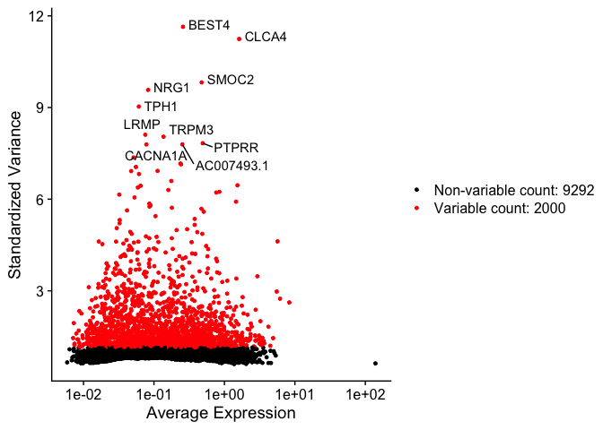
The function FindVariableFeatures identifies the most highly variable genes (default 2000 genes) by fitting a line to the relationship of log(variance) and log(mean) using loess smoothing, uses this information to standardize the data, then calculates the variance of the standardized data. This helps avoid selecting genes that only appear variable due to their expression level.
?FindVariableFeatures
experiment.aggregate <- FindVariableFeatures(
  object = experiment.aggregate,
  selection.method = "vst")
length(VariableFeatures(experiment.aggregate))
top10 <- head(VariableFeatures(experiment.aggregate), 10)
top10
var.feat.plot <- VariableFeaturePlot(experiment.aggregate)
var.feat.plot <- LabelPoints(plot = var.feat.plot, points = top10, repel = TRUE)
var.feat.plot
How do the results change if you use selection.method = “dispersion” or selection.method = “mean.var.plot”?
FindVariableFeatures isn’t the only way to set the “variable features” of a Seurat object. Another reasonable approach is to select a set of “minimally expressed” genes.
min.value <- 2
min.cells <- 10

num.cells <- Matrix::rowSums(GetAssayData(experiment.aggregate, slot = "count") > min.value)
genes.use <- names(num.cells[which(num.cells >= min.cells)])
length(genes.use)
VariableFeatures(experiment.aggregate) <- genes.use
Scale the data
The ScaleData function scales and centers genes in the dataset. If variables are provided with the “vars.to.regress” argument, they are individually regressed against each gene, and the resulting residuals are then scaled and centered unless otherwise specified. We regress out cell cycle results S.Score and G2M.Score, mitochondrial RNA level (percent_MT), and the number of features (nFeature_RNA) as a proxy for sequencing depth.
experiment.aggregate <- ScaleData(experiment.aggregate,
                                  vars.to.regress = c("S.Score", "G2M.Score", "percent_MT", "nFeature_RNA"))
Prepare for the next section
Save object
saveRDS(experiment.aggregate, file = "scRNA_workshop-03.rds")
Download Rmd
download.file("https://raw.githubusercontent.com/ucdavis-bioinformatics-training/2023-December-Single-Cell-RNA-Seq-Analysis/main/data_analysis/04-dimensionality_reduction.Rmd", "04-dimensionality_reduction.Rmd")
Session Information
sessionInfo()