Differential Gene Expression Analysis in R

• Differential Gene Expression (DGE) between conditions is determined from count data
• Generally speaking differential expression analysis is performed in a very similar manner to metabolomics, proteomics, or DNA microarrays, once normalization and transformations have been performed.

A lot of RNA-seq analysis has been done in R and so there are many packages available to analyze and view this data. Two of the most commonly used are:

• DESeq2, developed by Simon Anders (also created htseq) in Wolfgang Huber’s group at EMBL
• edgeR and Voom (extension to Limma [microarrays] for RNA-seq), developed out of Gordon Smyth’s group from the Walter and Eliza Hall Institute of Medical Research in Australia

http://bioconductor.org/packages/release/BiocViews.html#___RNASeq

Differential Expression Analysis with Limma-Voom

limma is an R package that was originally developed for differential expression (DE) analysis of gene expression microarray data.

voom is a function in the limma package that transforms RNA-Seq data for use with limma.

Together they allow fast, flexible, and powerful analyses of RNA-Seq data. Limma-voom is our tool of choice for DE analyses because it:

• Allows for incredibly flexible model specification (you can include multiple categorical and continuous variables, allowing incorporation of almost any kind of metadata).

• Based on simulation studies, maintains the false discovery rate at or below the nominal rate, unlike some other packages.

• Empirical Bayes smoothing of gene-wise standard deviations provides increased power.

Basic Steps of Differential Gene Expression

1. Read count data and annotation into R and preprocessing.
2. Calculate normalization factors (sample-specific adjustments)
3. Filter genes (uninteresting genes, e.g. unexpressed)
4. Account for expression-dependent variability by transformation, weighting, or modeling
5. Fitting a linear model
6. Perform statistical comparisons of interest (using contrasts)
7. Adjust for multiple testing, Benjamini-Hochberg (BH) or q-value
8. Check results for confidence
9. Attach annotation if available and write tables

1. Read in the counts table and create our DGEList

counts <- read.delim("rnaseq_workshop_counts.txt", row.names = 1)
head(counts)

Create Differential Gene Expression List Object (DGEList) object

A DGEList is an object in the package edgeR for storing count data, normalization factors, and other information

d0 <- DGEList(counts)

1a. Read in Annotation

anno <- read.delim("ensembl_mm_109.txt",as.is=T)
dim(anno)

head(anno)

tail(anno)

any(duplicated(anno$Gene.stable.ID))

1b. Derive experiment metadata from the sample names

Our experiment has two factors, genotype (“WT”, “KOMIR150”, or “KOTet3”) and cell type (“C” or “NC”).

The sample names are “mouse” followed by an animal identifier, followed by the genotype, followed by the cell type.

sample_names <- colnames(counts)
metadata <- as.data.frame(strsplit2(sample_names, c("_"))[,2:4], row.names = sample_names)
colnames(metadata) <- c("mouse", "genotype", "cell_type")

Create a new variable “group” that combines genotype and cell type.

metadata$group <- interaction(metadata$genotype, metadata$cell_type)
table(metadata$group)

table(metadata$mouse)

Note: you can also enter group information manually, or read it in from an external file. If you do this, it is $VERY, VERY, VERY$ important that you make sure the metadata is in the same order as the column names of the counts table.

Quiz 1

Submit Quiz

2. Preprocessing and Normalization factors

In differential expression analysis, only sample-specific effects need to be normalized, we are NOT concerned with comparisons and quantification of absolute expression.

• Sequence depth – is a sample specific effect and needs to be adjusted for.
• RNA composition - finding a set of scaling factors for the library sizes that minimize the log-fold changes between the samples for most genes (edgeR uses a trimmed mean of M-values between each pair of sample)
• GC content – is NOT sample-specific (except when it is)
• Gene Length – is NOT sample-specific (except when it is)

In edgeR/limma, you calculate normalization factors to scale the raw library sizes (number of reads) using the function calcNormFactors, which by default uses TMM (weighted trimmed means of M values to the reference). Assumes most genes are not DE.

Proposed by Robinson and Oshlack (2010).

d0 <- calcNormFactors(d0)
d0$samples

Note: calcNormFactors doesn’t normalize the data, it just calculates normalization factors for use downstream.

3. Filtering genes

We filter genes based on non-experimental factors to reduce the number of genes/tests being conducted and therefor do not have to be accounted for in our transformation or multiple testing correction. Commonly we try to remove genes that are either a) unexpressed, or b) unchanging (low-variability).

Common filters include:

1. to remove genes with a max value (X) of less then Y.
2. to remove genes that are less than X normalized read counts (cpm) across a certain number of samples. Ex: rowSums(cpms <=1) < 3 , require at least 1 cpm in at least 3 samples to keep.
3. A less used filter is for genes with minimum variance across all samples, so if a gene isn’t changing (constant expression) its inherently not interesting therefor no need to test.

We will use the built in function filterByExpr() to filter low-expressed genes. filterByExpr uses the experimental design to determine how many samples a gene needs to be expressed in to stay. Importantly, once this number of samples has been determined, the group information is not used in filtering.

Using filterByExpr requires specifying the model we will use to analysis our data.

• The model you use will change for every experiment, and this step should be given the most time and attention.*

We use a model that includes group and (in order to account for the paired design) mouse.

group <- metadata$group
mouse <- metadata$mouse
mm <- model.matrix(~0 + group + mouse)
head(mm)

keep <- filterByExpr(d0, mm)
sum(keep) # number of genes retained

d <- d0[keep,]

“Low-expressed” depends on the dataset and can be subjective.

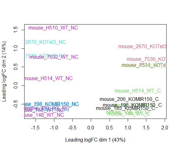
Visualizing your data with a Multidimensional scaling (MDS) plot.

plotMDS(d, col = as.numeric(metadata$group), cex=1)

The MDS plot tells you A LOT about what to expect from your experiment.

3a. Extracting “normalized” expression table

RPKM vs. FPKM vs. CPM and Model Based

• RPKM - Reads per kilobase per million mapped reads
• FPKM - Fragments per kilobase per million mapped reads
• logCPM – log Counts per million [ good for producing MDS plots, estimate of normalized values in model based ]
• Model based - original read counts are not themselves transformed, but rather correction factors are used in the DE model itself.

We use the cpm function with log=TRUE to obtain log-transformed normalized expression data. On the log scale, the data has less mean-dependent variability and is more suitable for plotting.

logcpm <- cpm(d, prior.count=2, log=TRUE)
write.table(logcpm,"rnaseq_workshop_normalized_counts.txt",sep="\t",quote=F)

Quiz 2

Submit Quiz

4. Voom transformation and calculation of variance weights

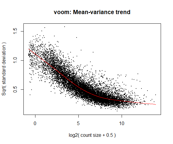
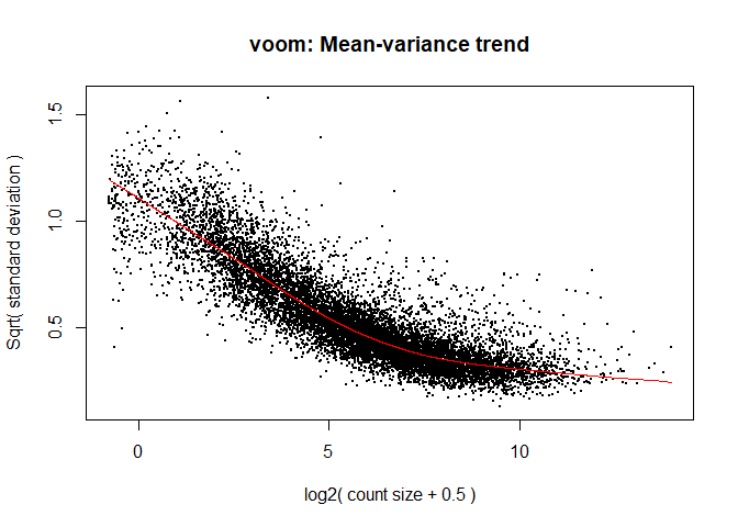
4a. Voom

y <- voom(d, mm, plot = T)

What is voom doing?

1. Counts are transformed to log2 counts per million reads (CPM), where “per million reads” is defined based on the normalization factors we calculated earlier.
2. A linear model is fitted to the log2 CPM for each gene, and the residuals are calculated.
3. A smoothed curve is fitted to the sqrt(residual standard deviation) by average expression. (see red line in plot above)
4. The smoothed curve is used to obtain weights for each gene and sample that are passed into limma along with the log2 CPMs.

More details at “voom: precision weights unlock linear model analysis tools for RNA-seq read counts”

If your voom plot looks like the below (performed on the raw data), you might want to filter more:

tmp <- voom(d0, mm, plot = T)

5. Fitting linear models in limma

lmFit fits a linear model using weighted least squares for each gene:

fit <- lmFit(y, mm)

head(coef(fit))

Comparisons between groups (log fold-changes) are obtained as contrasts of these fitted linear models:

6. Specify which groups to compare using contrasts:

Comparison between cell types for genotype WT.

contr <- makeContrasts(groupWT.C - groupWT.NC, levels = colnames(coef(fit)))
contr

6a. Estimate contrast for each gene

tmp <- contrasts.fit(fit, contr)

The variance characteristics of low expressed genes are different from high expressed genes, if treated the same, the effect is to over represent low expressed genes in the DE list. This is corrected for by the log transformation and voom. However, some genes will have increased or decreased variance that is not a result of low expression, but due to other random factors. We are going to run empirical Bayes to adjust the variance of these genes.

Empirical Bayes smoothing of standard errors (shifts standard errors that are much larger or smaller than those from other genes towards the average standard error) (see “Linear Models and Empirical Bayes Methods for Assessing Differential Expression in Microarray Experiments”

6b. Apply EBayes

tmp <- eBayes(tmp)

7. Multiple Testing Adjustment

The TopTable. Adjust for multiple testing using method of Benjamini & Hochberg (BH), or its ‘alias’ fdr. “Controlling the false discovery rate: a practical and powerful approach to multiple testing.

here n=Inf says to produce the topTable for all genes.

top.table <- topTable(tmp, adjust.method = "BH", sort.by = "P", n = Inf)

Multiple Testing Correction

Simply a must! Best choices are:

• FDR (false discovery rate), such as Benjamini-Hochberg (1995).
• Qvalue - Storey (2002)

The FDR (or qvalue) is a statement about the list and is no longer about the gene (pvalue). So a FDR of 0.05, says you expect 5% false positives among the list of genes with an FDR of 0.05 or less.

The statement “Statistically significantly different” means FDR of 0.05 or less.

7a. How many DE genes are there (false discovery rate corrected)?

length(which(top.table$adj.P.Val < 0.05))

8. Check your results for confidence.

You’ve conducted an experiment, you’ve seen a phenotype. Now check which genes are most differentially expressed (show the top 50)? Look up these top genes, their description and ensure they relate to your experiment/phenotype.

head(top.table, 50)

Columns are

• logFC: log2 fold change of WT.C/WT.NC
• AveExpr: Average expression across all samples, in log2 CPM
• t: logFC divided by its standard error
• P.Value: Raw p-value (based on t) from test that logFC differs from 0
• adj.P.Val: Benjamini-Hochberg false discovery rate adjusted p-value
• B: log-odds that gene is DE (arguably less useful than the other columns)

ENSMUSG00000030203.18 has higher expression at WT NC than at WT C (logFC is negative). ENSMUSG00000026193.16 has higher expression at WT C than at WT NC (logFC is positive).

9. Write top.table to a file, adding in cpms and annotation

top.table$Gene <- rownames(top.table)
top.table <- top.table[,c("Gene", names(top.table)[1:6])]
top.table <- data.frame(top.table,anno[match(top.table$Gene,anno$Gene.stable.ID.version),],logcpm[match(top.table$Gene,rownames(logcpm)),])

head(top.table)

write.table(top.table, file = "WT.C_v_WT.NC.txt", row.names = F, sep = "\t", quote = F)

Quiz 3

Submit Quiz

Linear models and contrasts

Let’s say we want to compare genotypes for cell type C. The only thing we have to change is the call to makeContrasts:

contr <- makeContrasts(groupWT.C - groupKOMIR150.C, levels = colnames(coef(fit)))
tmp <- contrasts.fit(fit, contr)
tmp <- eBayes(tmp)
top.table <- topTable(tmp, sort.by = "P", n = Inf)
head(top.table, 20)

length(which(top.table$adj.P.Val < 0.05)) # number of DE genes

top.table$Gene <- rownames(top.table)
top.table <- top.table[,c("Gene", names(top.table)[1:6])]
top.table <- data.frame(top.table,anno[match(top.table$Gene,anno$Gene.stable.ID),],logcpm[match(top.table$Gene,rownames(logcpm)),])

write.table(top.table, file = "WT.C_v_KOMIR150.C.txt", row.names = F, sep = "\t", quote = F)

What if we refit our model as a two-factor model (rather than using the group variable)?

Create new model matrix:

genotype <- factor(metadata$genotype, levels = c("WT", "KOMIR150", "KOTet3"))
cell_type <- factor(metadata$cell_type, levels = c("C", "NC"))
mouse <- factor(metadata$mouse, levels = c("110", "148", "158", "183", "198", "206", "2670", "7530", "7531", "7532", "H510", "H514"))
mm <- model.matrix(~genotype*cell_type + mouse)

We are specifying that model includes effects for genotype, cell type, and the genotype-cell type interaction (which allows the differences between genotypes to differ across cell types).

colnames(mm)

y <- voom(d, mm, plot = F)

fit <- lmFit(y, mm)

head(coef(fit))

colnames(coef(fit))

• The coefficient genotypeKOMIR150 represents the difference in mean expression between KOMIR150 and the reference genotype (WT), for cell type C (the reference level for cell type)
• The coefficient cell_typeNC represents the difference in mean expression between cell type NC and cell type C, for genotype WT
• The coefficient genotypeKOMIR150:cell_typeNC is the difference between cell types NC and C of the differences between genotypes KOMIR150 and WT (the interaction effect).

Let’s estimate the difference between genotypes WT and KOMIR150 in cell type C.

tmp <- contrasts.fit(fit, coef = 2) # Directly test second coefficient
tmp <- eBayes(tmp)
top.table <- topTable(tmp, sort.by = "P", n = Inf)
head(top.table, 20)

length(which(top.table$adj.P.Val < 0.05)) # number of DE genes

We get the same results as with the model where each coefficient corresponded to a group mean. In essence, these are the same model, so use whichever is most convenient for what you are estimating.

The interaction effects genotypeKOMIR150:cell_typeNC are easier to estimate and test in this setup.

head(coef(fit))

colnames(coef(fit))

tmp <- contrasts.fit(fit, coef = 16) # Test genotypeKOMIR150:cell_typeNC
tmp <- eBayes(tmp)
top.table <- topTable(tmp, sort.by = "P", n = Inf)
head(top.table, 20)

length(which(top.table$adj.P.Val < 0.05))

The log fold change here is the difference between genotypes KOMIR150 and WT in the log fold changes between cell types NC and C.

A gene for which this interaction effect is significant is one for which the effect of cell type differs between genotypes, and for which the effect of genotypes differs between cell types.

More complicated models

Specifying a different model is simply a matter of changing the calls to model.matrix (and possibly to contrasts.fit).

What if we want to adjust for a continuous variable like some health score? (We are making this data up here, but it would typically be a variable in your metadata.)

# Generate example health data
set.seed(99)
HScore <- rnorm(n = 22, mean = 7.5, sd = 1)
HScore

Model adjusting for HScore score:

mm <- model.matrix(~0 + group + mouse + HScore)
y <- voom(d, mm, plot = F)

fit <- lmFit(y, mm)

contr <- makeContrasts(groupKOMIR150.NC - groupWT.NC,
                       levels = colnames(coef(fit)))
tmp <- contrasts.fit(fit, contr)
tmp <- eBayes(tmp)
top.table <- topTable(tmp, sort.by = "P", n = Inf)
head(top.table, 20)

length(which(top.table$adj.P.Val < 0.05))

What if we want to look at the correlation of gene expression with a continuous variable like pH?

# Generate example pH data
set.seed(99)
pH <- rnorm(n = 22, mean = 8, sd = 1.5)
pH

Specify model matrix:

mm <- model.matrix(~pH)
head(mm)

y <- voom(d, mm, plot = F)
fit <- lmFit(y, mm)
tmp <- contrasts.fit(fit, coef = 2) # test "pH" coefficient
tmp <- eBayes(tmp)
top.table <- topTable(tmp, sort.by = "P", n = Inf)
head(top.table, 20)

length(which(top.table$adj.P.Val < 0.05))

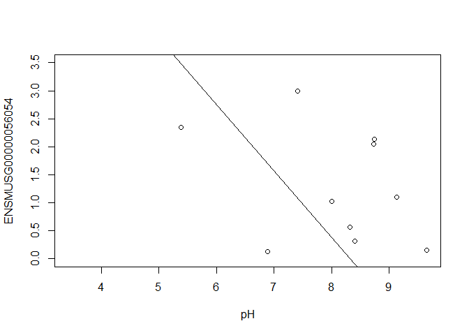
In this case, limma is fitting a linear regression model, which here is a straight line fit, with the slope and intercept defined by the model coefficients:

ENSMUSG00000056054 <- y$E["ENSMUSG00000056054.10",]
plot(ENSMUSG00000056054 ~ pH, ylim = c(0, 3.5))
intercept <- coef(fit)["ENSMUSG00000056054.10", "(Intercept)"]
slope <- coef(fit)["ENSMUSG00000056054.10", "pH"]
abline(a = intercept, b = slope)

slope

In this example, the log fold change logFC is the slope of the line, or the change in gene expression (on the log2 CPM scale) for each unit increase in pH.

Here, a logFC of 0.20 means a 0.20 log2 CPM increase in gene expression for each unit increase in pH, or a 15% increase on the CPM scale (2^0.20 = 1.15).

A bit more on linear models

Limma fits a linear model to each gene.

Linear models include analysis of variance (ANOVA) models, linear regression, and any model of the form

Y = β₀ + β₁X₁ + β₂X₂ + … + β_pX_p + ε

The covariates X can be:

• a continuous variable (pH, HScore score, age, weight, temperature, etc.)
• Dummy variables coding a categorical covariate (like cell type, genotype, and group)

The β’s are unknown parameters to be estimated.

In limma, the β’s are the log fold changes.

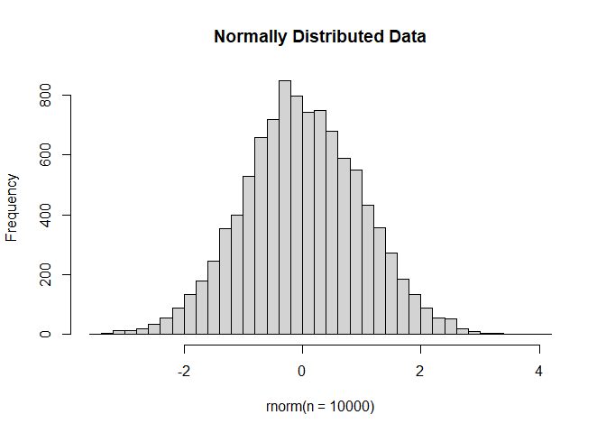
The error (residual) term ε is assumed to be normally distributed with a variance that is constant across the range of the data.

Normally distributed means the residuals come from a distribution that looks like this:

The log2 transformation that voom applies to the counts makes the data “normal enough”, but doesn’t completely stabilize the variance:

mm <- model.matrix(~0 + group + mouse)
tmp <- voom(d, mm, plot = T)

The log2 counts per million are more variable at lower expression levels. The variance weights calculated by voom address this situation.

Both edgeR and limma have VERY comprehensive user manuals

The limma users’ guide has great details on model specification.

• Limma voom

• edgeR

Simple plotting

mm <- model.matrix(~genotype*cell_type + mouse)
colnames(mm) <- make.names(colnames(mm))
y <- voom(d, mm, plot = F)

fit <- lmFit(y, mm)

contrast.matrix <- makeContrasts(genotypeKOMIR150, levels=colnames(coef(fit)))
fit2 <- contrasts.fit(fit, contrast.matrix)
fit2 <- eBayes(fit2)
top.table <- topTable(fit2, coef = 1, sort.by = "P", n = 40)

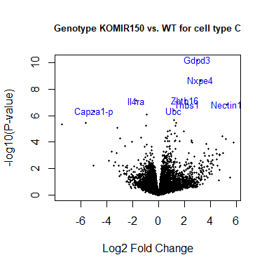
Volcano plot

volcanoplot(fit2, coef=1, highlight=8, names=rownames(fit2), main="Genotype KOMIR150 vs. WT for cell type C", cex.main = 0.8)

head(anno[match(rownames(fit2), anno$Gene.stable.ID.version),
     c("Gene.stable.ID.version", "Gene.name") ])

identical(anno[match(rownames(fit2), anno$Gene.stable.ID.version),
     c("Gene.stable.ID.version")], rownames(fit2))

volcanoplot(fit2, coef=1, highlight=8, names=anno[match(rownames(fit2), anno$Gene.stable.ID.version), "Gene.name"], main="Genotype KOMIR150 vs. WT for cell type C", cex.main = 0.8)

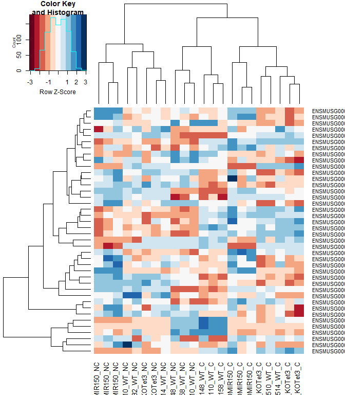
Heatmap

#using a red and blue color scheme without traces and scaling each row
heatmap.2(logcpm[rownames(top.table),],col=brewer.pal(11,"RdBu"),scale="row", trace="none")

anno[match(rownames(top.table), anno$Gene.stable.ID.version),
     c("Gene.stable.ID.version", "Gene.name")]

identical(anno[match(rownames(top.table), anno$Gene.stable.ID.version), "Gene.stable.ID.version"], rownames(top.table))

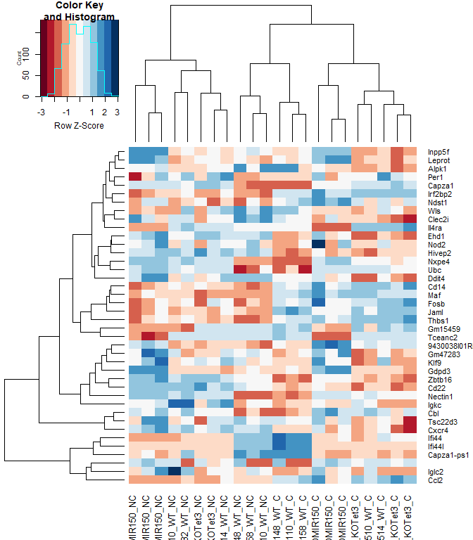
heatmap.2(logcpm[rownames(top.table),],col=brewer.pal(11,"RdBu"),scale="row", trace="none", labRow = anno[match(rownames(top.table), anno$Gene.stable.ID.version), "Gene.name"])

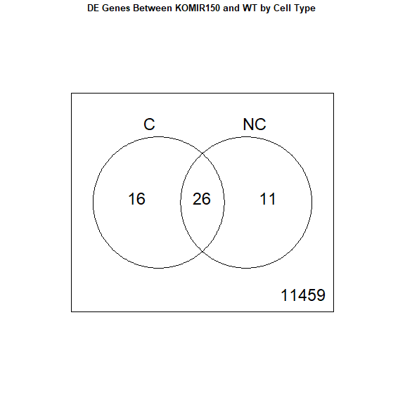
2 factor venn diagram

mm <- model.matrix(~genotype*cell_type + mouse)
colnames(mm) <- make.names(colnames(mm))
y <- voom(d, mm, plot = F)

fit <- lmFit(y, mm)

contrast.matrix <- makeContrasts(genotypeKOMIR150, genotypeKOMIR150 + genotypeKOMIR150.cell_typeNC, levels=colnames(coef(fit)))
fit2 <- contrasts.fit(fit, contrast.matrix)
fit2 <- eBayes(fit2)
top.table <- topTable(fit2, coef = 1, sort.by = "P", n = 40)

results <- decideTests(fit2)
vennDiagram(results, names = c("C", "NC"), main = "DE Genes Between KOMIR150 and WT by Cell Type", cex.main = 0.8)

Download the Enrichment Analysis R Markdown document

download.file("https://raw.githubusercontent.com/ucdavis-bioinformatics-training/2023-June-RNA-Seq-Analysis/master/data_analysis/enrichment_mm.Rmd", "enrichment_mm.Rmd")

sessionInfo()