GO AND KEGG Enrichment Analysis

Load libraries

library(topGO)
library(org.Mm.eg.db)
library(clusterProfiler)
library(pathview)
library(enrichplot)
library(ggplot2)
library(dplyr)

Files for examples were created in the DE analysis.

Gene Ontology (GO) Enrichment

Gene ontology provides a controlled vocabulary for describing biological processes (BP ontology), molecular functions (MF ontology) and cellular components (CC ontology)

The GO ontologies themselves are organism-independent; terms are associated with genes for a specific organism through direct experimentation or through sequence homology with another organism and its GO annotation.

Terms are related to other terms through parent-child relationships in a directed acylic graph.

Enrichment analysis provides one way of drawing conclusions about a set of differential expression results.

1. topGO Example Using Kolmogorov-Smirnov Testing Our first example uses Kolmogorov-Smirnov Testing for enrichment testing of our mouse DE results, with GO annotation obtained from the Bioconductor database org.Mm.eg.db.

The first step in each topGO analysis is to create a topGOdata object. This contains the genes, the score for each gene (here we use the p-value from the DE test), the GO terms associated with each gene, and the ontology to be used (here we use the biological process ontology)

infile <- "WT.C_v_WT.NC.txt"
DE <- read.delim(infile)

## Add entrezgene IDs to top table
tmp <- bitr(DE$Gene.stable.ID, fromType = "ENSEMBL", toType = "ENTREZID", OrgDb = org.Mm.eg.db)

id.conv <- subset(tmp, !duplicated(tmp$ENSEMBL))
DE <- left_join(DE, id.conv, by = c("Gene.stable.ID" = "ENSEMBL"))

# Make gene list
DE.nodupENTREZ <- subset(DE, !is.na(ENTREZID) & !duplicated(ENTREZID))
geneList <- DE.nodupENTREZ$P.Value
names(geneList) <- DE.nodupENTREZ$ENTREZID
head(geneList)

# Create topGOData object
GOdata <- new("topGOdata",
	ontology = "BP",
	allGenes = geneList,
	geneSelectionFun = function(x)x,
	annot = annFUN.org , mapping = "org.Mm.eg.db")

2. The topGOdata object is then used as input for enrichment testing:

# Kolmogorov-Smirnov testing
resultKS <- runTest(GOdata, algorithm = "weight01", statistic = "ks")

tab <- GenTable(GOdata, raw.p.value = resultKS, topNodes = length(resultKS@score), numChar = 120)

topGO by default preferentially tests more specific terms, utilizing the topology of the GO graph. The algorithms used are described in detail here.

head(tab, 15)

• Annotated: number of genes (in our gene list) that are annotated with the term
• Significant: n/a for this example, same as Annotated here
• Expected: n/a for this example, same as Annotated here
• raw.p.value: P-value from Kolomogorov-Smirnov test that DE p-values annotated with the term are smaller (i.e. more significant) than those not annotated with the term.

The Kolmogorov-Smirnov test directly compares two probability distributions based on their maximum distance.

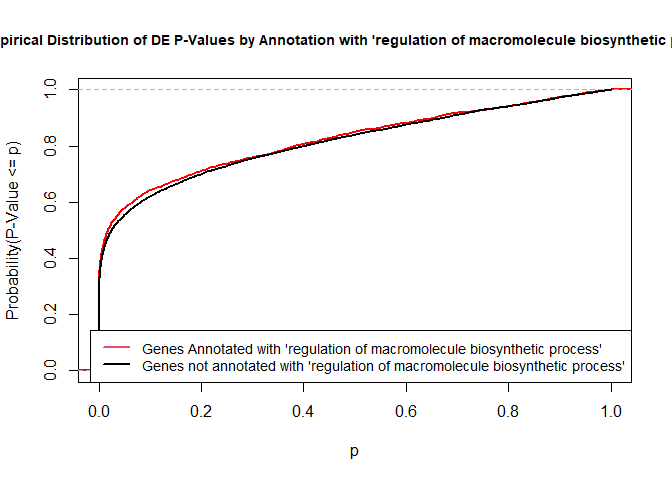
To illustrate the KS test, we plot probability distributions of p-values that are and that are not annotated with the term GO:0010556 “regulation of macromolecule biosynthetic process” (2344 genes) p-value 1.00. (This won’t exactly match what topGO does due to their elimination algorithm):

rna.pp.terms <- genesInTerm(GOdata)[["GO:0010556"]] # get genes associated with term
p.values.in <- geneList[names(geneList) %in% rna.pp.terms]
p.values.out <- geneList[!(names(geneList) %in% rna.pp.terms)]
plot.ecdf(p.values.in, verticals = T, do.points = F, col = "red", lwd = 2, xlim = c(0,1),
          main = "Empirical Distribution of DE P-Values by Annotation with 'regulation of macromolecule biosynthetic process'",
          cex.main = 0.9, xlab = "p", ylab = "Probability(P-Value <= p)")
ecdf.out <- ecdf(p.values.out)
xx <- unique(sort(c(seq(0, 1, length = 201), knots(ecdf.out))))
lines(xx, ecdf.out(xx), col = "black", lwd = 2)
legend("bottomright", legend = c("Genes Annotated with 'regulation of macromolecule biosynthetic process'", "Genes not annotated with 'regulation of macromolecule biosynthetic process'"), lwd = 2, col = 2:1, cex = 0.9)

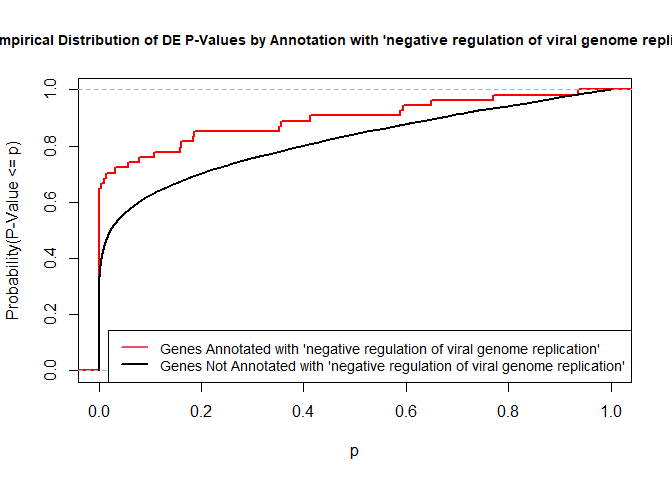
versus the probability distributions of p-values that are and that are not annotated with the term GO:0045071 “negative regulation of viral genome replication” (54 genes) p-value 3.3x10-9.

rna.pp.terms <- genesInTerm(GOdata)[["GO:0045071"]] # get genes associated with term
p.values.in <- geneList[names(geneList) %in% rna.pp.terms]
p.values.out <- geneList[!(names(geneList) %in% rna.pp.terms)]
plot.ecdf(p.values.in, verticals = T, do.points = F, col = "red", lwd = 2, xlim = c(0,1),
          main = "Empirical Distribution of DE P-Values by Annotation with 'negative regulation of viral genome replication'",
          cex.main = 0.9, xlab = "p", ylab = "Probability(P-Value <= p)")
ecdf.out <- ecdf(p.values.out)
xx <- unique(sort(c(seq(0, 1, length = 201), knots(ecdf.out))))
lines(xx, ecdf.out(xx), col = "black", lwd = 2)
legend("bottomright", legend = c("Genes Annotated with 'negative regulation of viral genome replication'", "Genes Not Annotated with 'negative regulation of viral genome replication'"), lwd = 2, col = 2:1, cex = 0.9)

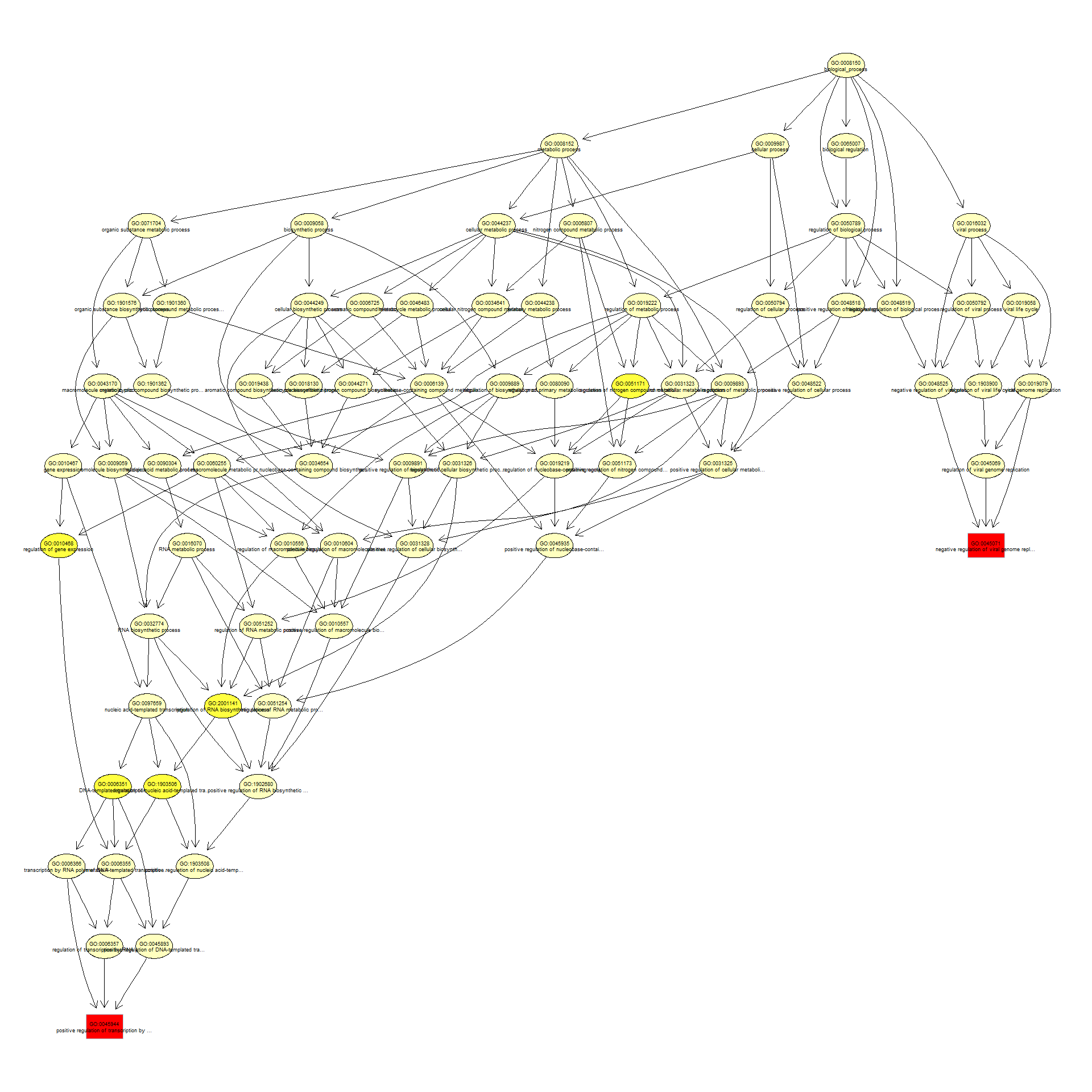
We can use the function showSigOfNodes to plot the GO graph for the 2 most significant terms and their parents, color coded by enrichment p-value (red is most significant):

par(cex = 0.3)
showSigOfNodes(GOdata, score(resultKS), firstSigNodes = 2, useInfo = "def", .NO.CHAR = 40)

par(cex = 1)

3. topGO Example Using Fisher’s Exact Test

Next, we use Fisher’s exact test to test for GO enrichment among significantly DE genes.

Create topGOdata object:

# Create topGOData object
GOdata <- new("topGOdata",
	ontology = "BP",
	allGenes = geneList,
	geneSelectionFun = function(x) (x < 0.05),
	annot = annFUN.org , mapping = "org.Mm.eg.db")

Run Fisher’s Exact Test:

resultFisher <- runTest(GOdata, algorithm = "elim", statistic = "fisher")

tab <- GenTable(GOdata, raw.p.value = resultFisher, topNodes = length(resultFisher@score),
				numChar = 120)
head(tab)

• Annotated: number of genes (in our gene list) that are annotated with the term
• Significant: Number of significantly DE genes annotated with that term (i.e. genes where geneList = 1)
• Expected: Under random chance, number of genes that would be expected to be significantly DE and annotated with that term
• raw.p.value: P-value from Fisher’s Exact Test, testing for association between significance and pathway membership.

Fisher’s Exact Test is applied to the table:

and compares the probability of the observed table, conditional on the row and column sums, to what would be expected under random chance.

Advantages over KS (or Wilcoxon) Tests:

• Ease of interpretation

• Can be applied when you just have a gene list without associated p-values, etc.

Disadvantages:

• Relies on significant/non-significant dichotomy (an interesting gene could have an adjusted p-value of 0.051 and be counted as non-significant)
• Less powerful
• May be less useful if there are very few (or a large number of) significant genes

Quiz 1

Submit Quiz

KEGG Pathway Enrichment Testing With clusterProfiler

KEGG, the Kyoto Encyclopedia of Genes and Genomes (https://www.genome.jp/kegg/), provides assignment of genes for many organisms into pathways.

We will conduct KEGG enrichment testing using the Bioconductor package clusterProfiler. clusterProfiler implements the algorithm used by GSEA.

Cluster profiler can do much more than KEGG enrichment, check out the clusterProfiler book.

We will base our KEGG enrichment analysis on the t statistics from differential expression, which allows for directional testing.

geneList.KEGG <- DE.nodupENTREZ$t                   
geneList.KEGG <- sort(geneList.KEGG, decreasing = TRUE)
names(geneList.KEGG) <- DE.nodupENTREZ$ENTREZID
head(geneList.KEGG)

KEGG.results <- gseKEGG(gene = geneList.KEGG, organism = "mmu", pvalueCutoff = 1)

KEGG.results <- setReadable(KEGG.results, OrgDb = "org.Mm.eg.db", keyType = "ENTREZID")
outdat <- as.data.frame(KEGG.results)
head(outdat)

Gene set enrichment analysis output includes the following columns:

• setSize: Number of genes in pathway

• enrichmentScore: GSEA enrichment score, a statistic reflecting the degree to which a pathway is overrepresented at the top or bottom of the gene list (the gene list here consists of the t-statistics from the DE test).

• NES: Normalized enrichment score

• pvalue: Raw p-value from permutation test of enrichment score

• p.adjust: Benjamini-Hochberg false discovery rate adjusted p-value

• qvalue: Storey false discovery rate adjusted p-value

• rank: Position in ranked list at which maximum enrichment score occurred

• leading_edge: Statistics from leading edge analysis

Dotplot of enrichment results

Gene.ratio = (count of core enrichment genes)/(count of pathway genes)

Core enrichment genes = subset of genes that contribute most to the enrichment result (“leading edge subset”)

dotplot(KEGG.results)

Pathview plot of log fold changes on KEGG diagram

foldChangeList <- DE$logFC
xx <- as.list(org.Mm.egENSEMBL2EG)
names(foldChangeList) <- xx[sapply(strsplit(DE$Gene,split="\\."),"[[", 1L)]
head(foldChangeList)

mmu04015 <- pathview(gene.data  = foldChangeList,
                     pathway.id = "mmu04015",
                     species    = "mmu",
                     limit      = list(gene=max(abs(foldChangeList)), cpd=1))

Barplot of p-values for top pathways

A barplot of -log10(p-value) for the top pathways/terms can be used for any type of enrichment analysis.

plotdat <- outdat[1:10,]
plotdat$nice.name <- gsub(" - Mus musculus (house mouse)", "", plotdat$Description, fixed = TRUE)

ggplot(plotdat, aes(x = -log10(p.adjust), y = reorder(nice.name, -log10(p.adjust)), fill = setSize)) + geom_bar(stat = "identity") + labs(x = "-log10(P-Value)", y = NULL, fill = "# Genes") + scale_fill_gradient(low = "red", high = "blue")

Quiz 2

Submit Quiz

sessionInfo()