
RStudio and R notebooks
While all of the code functions from the command line, we recommend using RStudio for these course materials.
Launch RStudio.
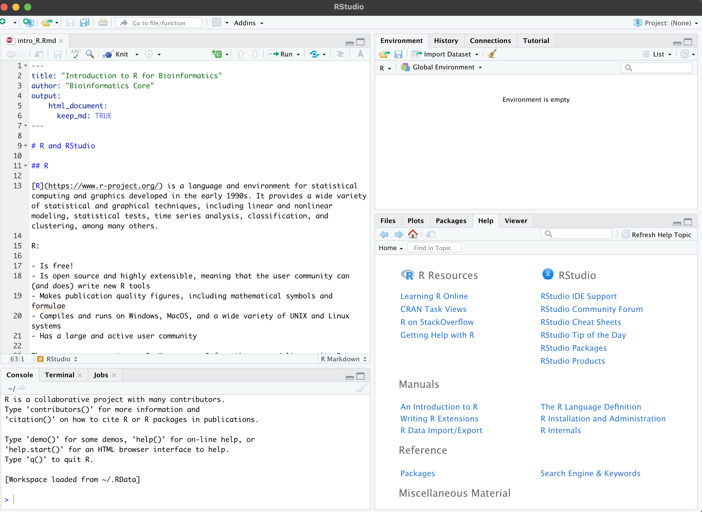
RStudio
RStudio is a convenient integrated development environment (IDE) for R. It provides a number of features that improve the experience of learning to the basics of R.
Your RStudio window should look something like this:
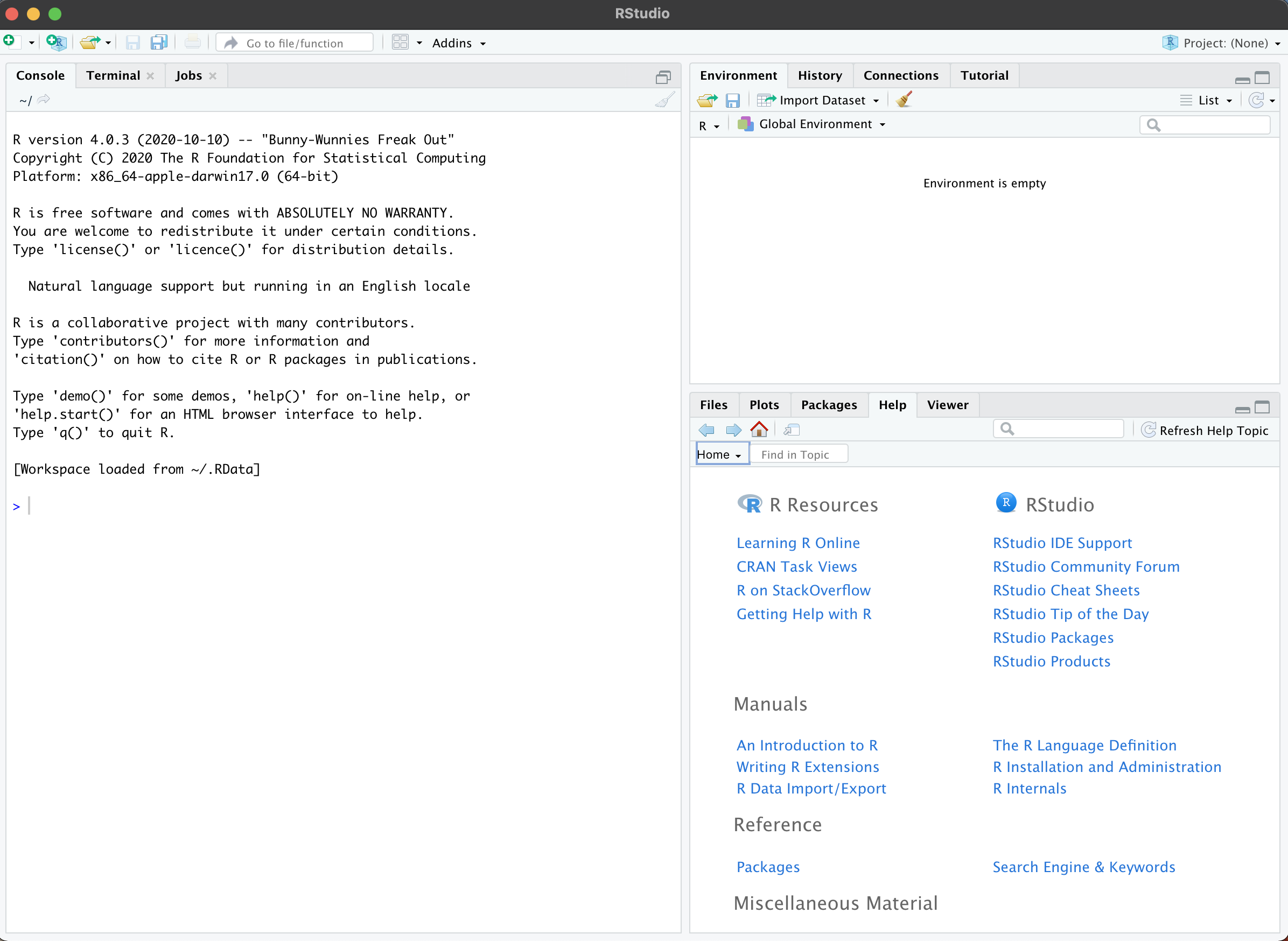
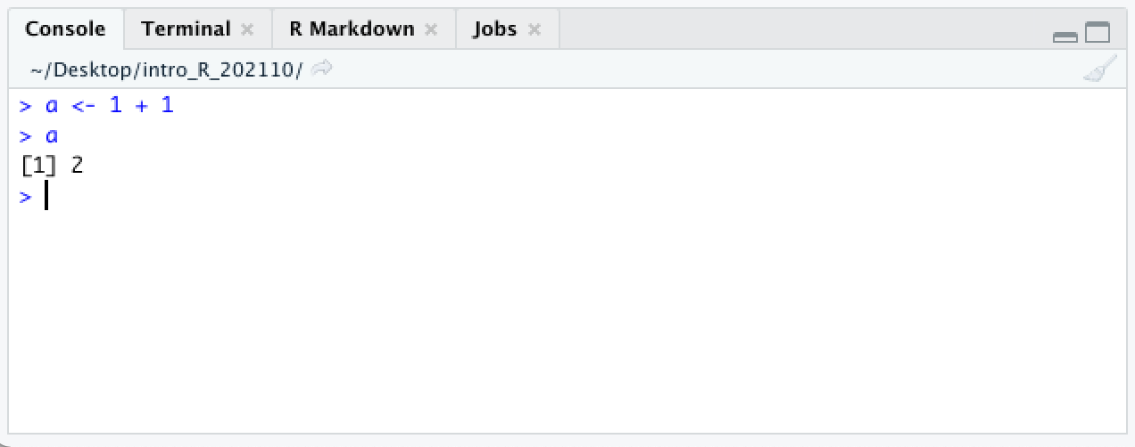
The console
On the left hand side is the console. This is a command-line interface for R. Type a command, press enter to run it, and the result appears below.
 For now, ignore the
 [1] at the beginning of the line. We will come back to it in a later section.
In R, the prompt is a > character. At the beginning of the line, it indicates that R is ready for your next command.
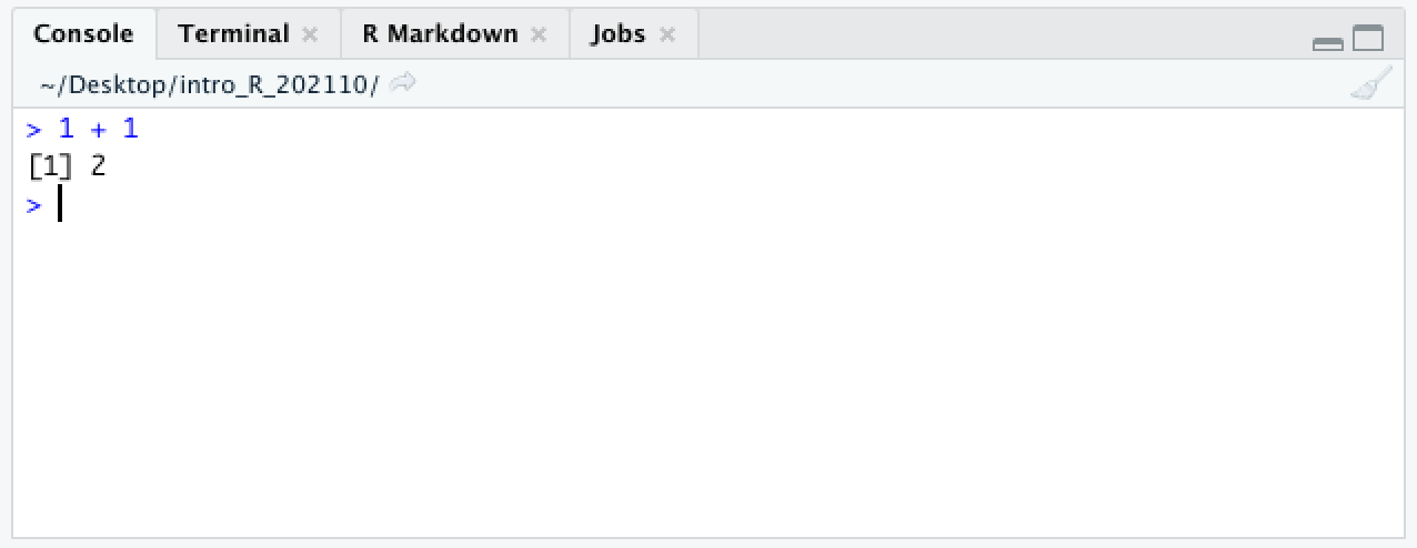
In these materials, code appears in gray boxes, like this:
1 + 1
Whenever you see one of these boxes, run the code yourself.
What happens if you press enter before you meant to?
1 +
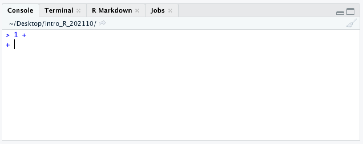
If you press enter before finishing a command, the next line will begin with a + character. This lets you know that R is expecting more input.
The workspace browser
In the upper right panel is the workspace (or environment) browser. This window shows the objects present in the environment. Currently there are none.
Objects are data stored in memory. The following code adds an object to the workspace.
a <- 1 + 1
Run the code in the gray box above.
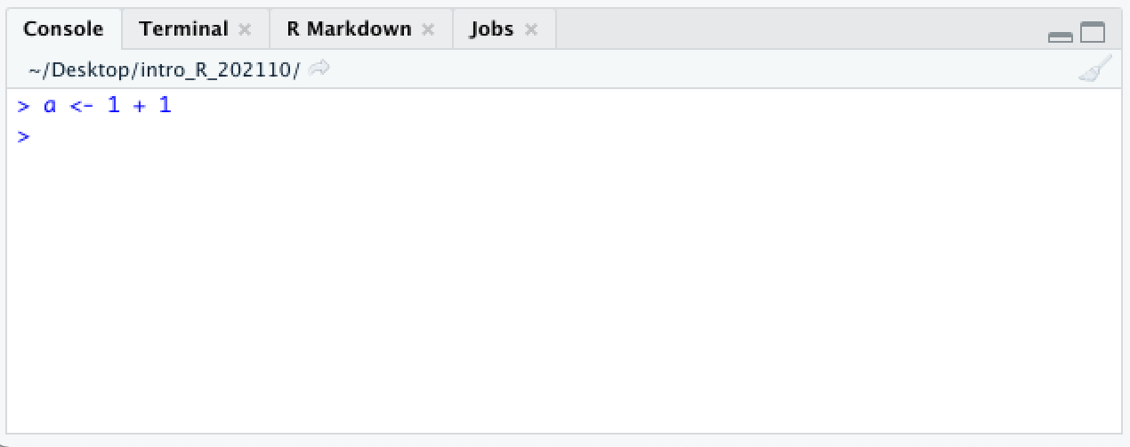
Unlike the first time we ran 1 + 1, nothing is printed to the console.
 Instead, a new value appears in the workspace browser.
Why? The <- is a special pair of characters called the assignment operator that stores the result of the addition in the object referred to on the left-hand side of the “arrow.” If no object with the name exists, one is created.
R evaluates the object and returns its value, 2. Objects retain their values until removed or reassigned.
The <- character pair is one of two assignment operators in R. In most situations, it is equivalent to the = character, but there are some exceptions, which we will address when they come up. This documentation follows the R convention of using <- in most cases.
Help documentation
The lower right pane contains the file browser, plot viewer, and help documentation, which we will be using frequently.
R notebooks
Create a new R notebook using the menu bar at the top: File > New File > R Notebook.
A fourth pane will open up containing a template R notebook. It should look something like this:
R notebooks are a special type of markdown document. They combine executable code, its output, and text. Markdown syntax is used to encode formatting like headings, bold or italic fonts, bullet points, links, and more. Using an R notebook keeps code, figures, and written commentary together, making it easy to generate a report with a single click.
Within a notebook, code is organized into chunks, which separates the text R will evaluate from any notes or images included in the notebook.
New chunks are added by clicking the Insert Chunk button on the toolbar or by pressing Ctrl+Alt+I on Windows, or Cmd+Option+I on Mac.
Code chunks are executed by clicking the Run button within the chunk or by placing your cursor inside it and pressing Ctrl+Shift+Enter on Windows, or Cmd+Shift+Enter on Mac. You can run a single line of code by placing your cursor anywhere on the line and pressing Ctrl+Enter on Windows, or Cmd+Enter on Mac.
Create and run a new chunk with the following code:
2 + 2
b <- 3 + 3
What happened? Where did the output for each line of code go?
Set up a folder for the course, and save your notebook.
Create a folder to contain all of the files for this course.
Directories (folders) and the files they contain should be named without spaces or special characters. Using only alphanumeric characters, dots, dashes, and underscores ensures that most programming languages will be able to understand the name of your file without any problems. If you use special characters like dollar signs, slashes, quotation marks, spaces, or parentheses, this is not always the case.
Save your R notebook to your new folder.
Importing and exporting data
For the remainder of this course, we will be working with a single data set to answer a number of simple biological questions about the effects of maternal cigarette use during pregnancy. This data is a table of parental and newborn birth weights adapted from a data set provided by Mathematics and Statistics Help at the University of Sheffield. It has been slightly modified to allow us to demonstrate a few more functions, but the data is largely unchanged.
Begin by setting up a working directory for this course.
We’re going to do all the work for this course in the directory we created in the last section. To make things easier, we’ll set R’s working directory to the directory where we saved our notebook. To do this, select the “Session” menu in the toolbar, then navigate to “Set Working Directory,” and click on “Choose Directory.” Choose the directory in which you saved your notebook.
When you do so, you should see that a line of code ran in your console:
setwd("/Users/hannah/Desktop/intro_R/")
This is the GUI at work! When you clicked on a directory in the file browser, R was actually running the code displayed in your console. In the future, you can set your working directory that way instead.
Download the data.
download.file("https://raw.githubusercontent.com/ucdavis-bioinformatics-training/2022_February_Introduction_to_R_for_Bioinformatics/main/birthweight.csv", "birthweight.csv")
Import data using read.csv()
Manual data entry is time-consuming and leads to errors. R has a number of functions for reading data in a variety of formats. Let’s use the read.csv() function to read in a spreadsheet containing data from an experiment.
birthweight <- read.csv("birthweight.csv")
CSV stands for “comma separated value,” and the CSV file is simply a text file where each row in the file represents a row in the data table, and the columns are separated by commas. The contents of the CSV file are now stored in the variable “birthweight.”
Export data using write.csv()
In the course of our analysis, we will add metrics to this data set. When we’re finished, we will want to be able to save our analyses. To write the contents of the birthweight object to a new CSV, we can use the write.csv() function.
write.csv(birthweight, file = "new_birthweight.csv")
The similar read.delim() and write.delim() can be used to read and write tab-delimited files, where columns are separated by tab characters rather than commas.
Data frames
Structure of a data frame
What is the birthweight object? In the environment browser, you should see that it is “42 obs. of 18 variables.” It’s probably a data table with 42 rows and 18 columns. We can verify this using the class() and dim() functions.
class(birthweight)
## [1] "data.frame"
dim(birthweight)
## [1] 42 18
A note on formatting: In this documentation lines beginning with ## are the output of the R code shown. Running dim(birthweight) asked R what the dimensions of the birthweight object are; the answer is 42 (rows) x 21 (columns). The “[1]” is not part of the output. It is an index added by R to help you keep track of the values when an operation outputs a large number of values. We will see other examples later that will hopefully make this more clear. For now, we can safely ignore that “[1]”.
A data frame organizes data into rows and columns. The object must be “rectangular,” with all rows having the same number of fields, and all values in a column must be of the same type.
Each column of a data frame is a vector. A vector is an ordered collection of values of the same type.
Let’s take a look at the contents.
birthweight
| ID | birth.date | location | length | birthweight | head.circumference | weeks.gestation | smoker | maternal.age | maternal.cigarettes | maternal.height | maternal.prepregnant.weight | paternal.age | paternal.education | paternal.cigarettes | paternal.height | low.birthweight | geriatric.pregnancy |
|---|---|---|---|---|---|---|---|---|---|---|---|---|---|---|---|---|---|
| 1107 | 1/25/1967 | General | 52 | 3.23 | 36 | 38 | no | 31 | 0 | 164 | 57 | NA | NA | NA | NA | 0 | FALSE |
| 697 | 2/6/1967 | Silver Hill | 48 | 3.03 | 35 | 39 | no | 27 | 0 | 162 | 62 | 27 | 14 | 0 | 178 | 0 | FALSE |
| 1683 | 2/14/1967 | Silver Hill | 53 | 3.35 | 33 | 41 | no | 27 | 0 | 164 | 62 | 37 | 14 | 0 | 170 | 0 | FALSE |
| 27 | 3/9/1967 | Silver Hill | 53 | 3.55 | 37 | 41 | yes | 37 | 25 | 161 | 66 | 46 | NA | 0 | 175 | 0 | TRUE |
| 1522 | 3/13/1967 | Memorial | 50 | 2.74 | 33 | 39 | yes | 21 | 17 | 156 | 53 | 24 | 12 | 7 | 179 | 0 | FALSE |
| 569 | 3/23/1967 | Memorial | 50 | 2.51 | 35 | 39 | yes | 22 | 7 | 159 | 52 | 23 | 14 | 25 | NA | 1 | FALSE |
| 365 | 4/23/1967 | Memorial | 52 | 3.53 | 37 | 40 | yes | 26 | 25 | 170 | 62 | 30 | 10 | 25 | 181 | 0 | FALSE |
| 808 | 5/5/1967 | Silver Hill | 48 | 2.92 | 33 | 34 | no | 26 | 0 | 167 | 64 | 25 | 12 | 25 | 175 | 0 | FALSE |
| 1369 | 6/4/1967 | Silver Hill | 49 | 3.18 | 34 | 38 | yes | 31 | 25 | 162 | 57 | 32 | 16 | 50 | 194 | 0 | FALSE |
| 1023 | 6/7/1967 | Memorial | 52 | 3.00 | 35 | 38 | yes | 30 | 12 | 165 | 64 | 38 | 14 | 50 | 180 | 0 | FALSE |
| 822 | 6/14/1967 | Memorial | 50 | 3.42 | 35 | 38 | no | 20 | 0 | 157 | 48 | 22 | 14 | 0 | 179 | 0 | FALSE |
| 1272 | 6/20/1967 | Memorial | 53 | 2.75 | 32 | 40 | yes | 37 | 50 | 168 | 61 | 31 | 16 | 0 | 173 | 0 | TRUE |
| 1262 | 6/25/1967 | Silver Hill | 53 | 3.19 | 34 | 41 | yes | 27 | 35 | 163 | 51 | 31 | 16 | 25 | 185 | 0 | FALSE |
| 575 | 7/12/1967 | Memorial | 50 | 2.78 | 30 | 37 | yes | 19 | 7 | 165 | 60 | 20 | 14 | 0 | 183 | 0 | FALSE |
| 1016 | 7/13/1967 | Silver Hill | 53 | 4.32 | 36 | 40 | no | 19 | 0 | 171 | 62 | 19 | 12 | 0 | 183 | 0 | FALSE |
| 792 | 9/7/1967 | Memorial | 53 | 3.64 | 38 | 40 | yes | 20 | 2 | 170 | 59 | 24 | 12 | 12 | 185 | 0 | FALSE |
| 820 | 10/7/1967 | General | 52 | 3.77 | 34 | 40 | no | 24 | 0 | 157 | 50 | 31 | 16 | 0 | 173 | 0 | FALSE |
| 752 | 10/19/1967 | General | 49 | 3.32 | 36 | 40 | yes | 27 | 12 | 152 | 48 | 37 | 12 | 25 | 170 | 0 | FALSE |
| 619 | 11/1/1967 | Memorial | 52 | 3.41 | 33 | 39 | yes | 23 | 25 | 181 | 69 | 23 | 16 | 2 | 181 | 0 | FALSE |
| 1764 | 12/7/1967 | Silver Hill | 58 | 4.57 | 39 | 41 | yes | 32 | 12 | 173 | 70 | 38 | 14 | 25 | 180 | 0 | FALSE |
| 1081 | 12/14/1967 | Silver Hill | 54 | 3.63 | 38 | 38 | no | 18 | 0 | 172 | 50 | 20 | 12 | 7 | 172 | 0 | FALSE |
| 516 | 1/8/1968 | Silver Hill | 47 | 2.66 | 33 | 35 | yes | 20 | 35 | 170 | 57 | 23 | 12 | 50 | 186 | 1 | FALSE |
| 272 | 1/10/1968 | Memorial | 52 | 3.86 | 36 | 39 | yes | 30 | 25 | 170 | 78 | 40 | 16 | 50 | 178 | 0 | FALSE |
| 321 | 1/21/1968 | Silver Hill | 48 | 3.11 | 33 | 37 | no | 28 | 0 | 158 | 54 | 39 | 10 | 0 | 171 | 0 | FALSE |
| 1636 | 2/2/1968 | Silver Hill | 51 | 3.93 | 38 | 38 | no | 29 | 0 | 165 | 61 | NA | NA | NA | NA | 0 | FALSE |
| 1360 | 2/16/1968 | General | 56 | 4.55 | 34 | 44 | no | 20 | 0 | 162 | 57 | 23 | 10 | 35 | 179 | 0 | FALSE |
| 1388 | 2/22/1968 | Memorial | 51 | 3.14 | 33 | 41 | yes | 22 | 7 | 160 | 53 | 24 | 16 | 12 | 176 | 0 | FALSE |
| 1363 | 4/2/1968 | General | 48 | 2.37 | 30 | 37 | yes | 20 | 7 | 163 | 47 | 20 | 10 | 35 | 185 | 1 | FALSE |
| 1058 | 4/24/1968 | Silver Hill | 53 | 3.15 | 34 | 40 | no | 29 | 0 | 167 | 60 | 30 | 16 | NA | 182 | 0 | FALSE |
| 755 | 4/25/1968 | Memorial | 53 | 3.20 | 33 | 41 | no | 21 | 0 | 155 | 55 | 25 | 14 | 25 | 183 | 0 | FALSE |
| 462 | 6/19/1968 | Silver Hill | 58 | 4.10 | 39 | 41 | no | 35 | 0 | 172 | 58 | 31 | 16 | 25 | 185 | 0 | TRUE |
| 300 | 7/18/1968 | Silver Hill | 46 | 2.05 | 32 | 35 | yes | 41 | 7 | 166 | 57 | 37 | 14 | 25 | 173 | 1 | TRUE |
| 1088 | 7/24/1968 | General | 51 | 3.27 | 36 | 40 | no | 24 | 0 | 168 | 53 | 29 | 16 | 0 | 181 | 0 | FALSE |
| 57 | 8/12/1968 | Memorial | 51 | 3.32 | 38 | 39 | yes | 23 | 17 | 157 | 48 | NA | NA | NA | NA | 0 | FALSE |
| 553 | 8/17/1968 | Silver Hill | 54 | 3.94 | 37 | 42 | no | 24 | 0 | 175 | 66 | 30 | 12 | 0 | 184 | 0 | FALSE |
| 1191 | 9/7/1968 | General | 53 | 3.65 | 33 | 42 | no | 21 | 0 | 165 | 61 | 21 | 10 | 25 | 185 | 0 | FALSE |
| 431 | 9/16/1968 | Silver Hill | 48 | 1.92 | 30 | 33 | yes | 20 | 7 | 161 | 50 | 20 | 10 | 35 | 180 | 1 | FALSE |
| 1313 | 9/27/1968 | Silver Hill | 43 | 2.65 | 32 | 33 | no | 24 | 0 | 149 | 45 | 26 | 16 | 0 | 169 | 1 | FALSE |
| 1600 | 10/9/1968 | General | 53 | 2.90 | 34 | 39 | no | 19 | 0 | 165 | 57 | NA | NA | NA | NA | 0 | FALSE |
| 532 | 10/25/1968 | General | 53 | 3.59 | 34 | 40 | yes | 31 | 12 | 163 | 49 | 41 | 12 | 50 | 191 | 0 | FALSE |
| 223 | 12/11/1968 | General | 50 | 3.87 | 33 | 45 | yes | 28 | 25 | 163 | 54 | 30 | 16 | 0 | 183 | 0 | FALSE |
| 1187 | 12/19/1968 | Silver Hill | 53 | 4.07 | 38 | 44 | no | 20 | 0 | 174 | 68 | 26 | 14 | 25 | 189 | 0 | FALSE |
The data frame format should look familiar. It’s a lot like a spreadsheet.
Generally, we don’t want to operate on the entire data frame. For example, to calculate the mean birth weight, we don’t need the information in the “paternal.education” column.
There are three ways to have R subset the data frame: $, [[, and [.
Selecting a single column using the $ and [[ operators
The simplest way to get all the values in the “birthweight” column is with the $ operator.
birthweight$birthweight
##  [1] 3.23 3.03 3.35 3.55 2.74 2.51 3.53 2.92 3.18 3.00 3.42 2.75 3.19 2.78 4.32
## [16] 3.64 3.77 3.32 3.41 4.57 3.63 2.66 3.86 3.11 3.93 4.55 3.14 2.37 3.15 3.20
## [31] 4.10 2.05 3.27 3.32 3.94 3.65 1.92 2.65 2.90 3.59 3.87 4.07
Notice that there are now three numbers inside brackets: one at the beginning of each line of output. These are the indices (locations) of the following number within the output vector. They give us a general idea of the length of the vector, and allow us to determine the value of a particular observation at a glance. For example, we can answer the question “what was the birth weight of the 34th baby?”
Once the vector of birth weights has been extracted from the rest of the data frame, it can be used to calculate a mean.
mean(birthweight$birthweight)
## [1] 3.312857
This $ operator is a shortcut for the [[ sub-setting operator, which requires typing six characters (two pairs of square brackets and a pair of quotation marks) rather than just one (the dollar sign). They function in the same way, returning the value of the element named.
birthweight[["birthweight"]]
##  [1] 3.23 3.03 3.35 3.55 2.74 2.51 3.53 2.92 3.18 3.00 3.42 2.75 3.19 2.78 4.32
## [16] 3.64 3.77 3.32 3.41 4.57 3.63 2.66 3.86 3.11 3.93 4.55 3.14 2.37 3.15 3.20
## [31] 4.10 2.05 3.27 3.32 3.94 3.65 1.92 2.65 2.90 3.59 3.87 4.07
mean(birthweight[["birthweight"]])
## [1] 3.312857
One difference to note is that while [[ works with the index, or column number, $ does not.
# which column contains the birth weight?
# lines beginning with a '#' are comments, and are not executed by R
colnames(birthweight)
##  [1] "ID"                          "birth.date"
##  [3] "location"                    "length"
##  [5] "birthweight"                 "head.circumference"
##  [7] "weeks.gestation"             "smoker"
##  [9] "maternal.age"                "maternal.cigarettes"
## [11] "maternal.height"             "maternal.prepregnant.weight"
## [13] "paternal.age"                "paternal.education"
## [15] "paternal.cigarettes"         "paternal.height"
## [17] "low.birthweight"             "geriatric.pregnancy"
birthweight[[5]]
##  [1] 3.23 3.03 3.35 3.55 2.74 2.51 3.53 2.92 3.18 3.00 3.42 2.75 3.19 2.78 4.32
## [16] 3.64 3.77 3.32 3.41 4.57 3.63 2.66 3.86 3.11 3.93 4.55 3.14 2.37 3.15 3.20
## [31] 4.10 2.05 3.27 3.32 3.94 3.65 1.92 2.65 2.90 3.59 3.87 4.07
mean(birthweight[[5]])
## [1] 3.312857
# the $ operator can't take an index
birthweight$5
Selecting a subset of the data frame using the [ operator
Unlike $ and [[, which return the value(s) contained in the specified element, [ returns an object of the same type it is used to subset. Using [ to retrieve the fifth column will return a data frame with 42 rows and 1 column. This may not seem like a big difference, but it can be an important distinction in some cases.
birthweight[5]
| birthweight |
|---|
| 3.23 |
| 3.03 |
| 3.35 |
| 3.55 |
| 2.74 |
| 2.51 |
| 3.53 |
| 2.92 |
| 3.18 |
| 3.00 |
| 3.42 |
| 2.75 |
| 3.19 |
| 2.78 |
| 4.32 |
| 3.64 |
| 3.77 |
| 3.32 |
| 3.41 |
| 4.57 |
| 3.63 |
| 2.66 |
| 3.86 |
| 3.11 |
| 3.93 |
| 4.55 |
| 3.14 |
| 2.37 |
| 3.15 |
| 3.20 |
| 4.10 |
| 2.05 |
| 3.27 |
| 3.32 |
| 3.94 |
| 3.65 |
| 1.92 |
| 2.65 |
| 2.90 |
| 3.59 |
| 3.87 |
| 4.07 |
Because the [ operator returns a new data frame, it can be used to specify multiple rows and / or columns.
birthweight[c(1,5)]
| ID | birthweight |
|---|---|
| 1107 | 3.23 |
| 697 | 3.03 |
| 1683 | 3.35 |
| 27 | 3.55 |
| 1522 | 2.74 |
| 569 | 2.51 |
| 365 | 3.53 |
| 808 | 2.92 |
| 1369 | 3.18 |
| 1023 | 3.00 |
| 822 | 3.42 |
| 1272 | 2.75 |
| 1262 | 3.19 |
| 575 | 2.78 |
| 1016 | 4.32 |
| 792 | 3.64 |
| 820 | 3.77 |
| 752 | 3.32 |
| 619 | 3.41 |
| 1764 | 4.57 |
| 1081 | 3.63 |
| 516 | 2.66 |
| 272 | 3.86 |
| 321 | 3.11 |
| 1636 | 3.93 |
| 1360 | 4.55 |
| 1388 | 3.14 |
| 1363 | 2.37 |
| 1058 | 3.15 |
| 755 | 3.20 |
| 462 | 4.10 |
| 300 | 2.05 |
| 1088 | 3.27 |
| 57 | 3.32 |
| 553 | 3.94 |
| 1191 | 3.65 |
| 431 | 1.92 |
| 1313 | 2.65 |
| 1600 | 2.90 |
| 532 | 3.59 |
| 223 | 3.87 |
| 1187 | 4.07 |
The c() function creates a vector. This allows R to treat indices 1 and 5 as a single argument. This is critical, because birthweight[1,5] does not produce the same effect at all.
birthweight[1, 5]
## [1] 3.23
What happened?
When there are two arguments provided to [, R interprets these as the index on the first (row) and second (column) dimension of the object. The value returned is the content of the first row, fifth column: the birth weight of individual 1107.
The default behavior of [ is to return the entire object. The first argument acts as a sort of filter on the first dimension, the second argument as a filter on the second dimension, and so on. Leaving the space before the comma blank will return all rows (no filter applied), while leaving the space following the comma blank will return all columns. Be sure to try variations on the example code below to see what happens.
birthweight[c(2,7,29), c(1,5)]
| ID | birthweight | |
|---|---|---|
| 2 | 697 | 3.03 |
| 7 | 365 | 3.53 |
| 29 | 1058 | 3.15 |
Using a minus sign before an index or group of indices will exclude the specified rows / columns.
colnames(birthweight)
##  [1] "ID"                          "birth.date"
##  [3] "location"                    "length"
##  [5] "birthweight"                 "head.circumference"
##  [7] "weeks.gestation"             "smoker"
##  [9] "maternal.age"                "maternal.cigarettes"
## [11] "maternal.height"             "maternal.prepregnant.weight"
## [13] "paternal.age"                "paternal.education"
## [15] "paternal.cigarettes"         "paternal.height"
## [17] "low.birthweight"             "geriatric.pregnancy"
# exclude paternal data (columns 13-16)
birthweight[c(1,3,5:13), -c(13:16)]
| ID | birth.date | location | length | birthweight | head.circumference | weeks.gestation | smoker | maternal.age | maternal.cigarettes | maternal.height | maternal.prepregnant.weight | low.birthweight | geriatric.pregnancy | |
|---|---|---|---|---|---|---|---|---|---|---|---|---|---|---|
| 1 | 1107 | 1/25/1967 | General | 52 | 3.23 | 36 | 38 | no | 31 | 0 | 164 | 57 | 0 | FALSE |
| 3 | 1683 | 2/14/1967 | Silver Hill | 53 | 3.35 | 33 | 41 | no | 27 | 0 | 164 | 62 | 0 | FALSE |
| 5 | 1522 | 3/13/1967 | Memorial | 50 | 2.74 | 33 | 39 | yes | 21 | 17 | 156 | 53 | 0 | FALSE |
| 6 | 569 | 3/23/1967 | Memorial | 50 | 2.51 | 35 | 39 | yes | 22 | 7 | 159 | 52 | 1 | FALSE |
| 7 | 365 | 4/23/1967 | Memorial | 52 | 3.53 | 37 | 40 | yes | 26 | 25 | 170 | 62 | 0 | FALSE |
| 8 | 808 | 5/5/1967 | Silver Hill | 48 | 2.92 | 33 | 34 | no | 26 | 0 | 167 | 64 | 0 | FALSE |
| 9 | 1369 | 6/4/1967 | Silver Hill | 49 | 3.18 | 34 | 38 | yes | 31 | 25 | 162 | 57 | 0 | FALSE |
| 10 | 1023 | 6/7/1967 | Memorial | 52 | 3.00 | 35 | 38 | yes | 30 | 12 | 165 | 64 | 0 | FALSE |
| 11 | 822 | 6/14/1967 | Memorial | 50 | 3.42 | 35 | 38 | no | 20 | 0 | 157 | 48 | 0 | FALSE |
| 12 | 1272 | 6/20/1967 | Memorial | 53 | 2.75 | 32 | 40 | yes | 37 | 50 | 168 | 61 | 0 | TRUE |
| 13 | 1262 | 6/25/1967 | Silver Hill | 53 | 3.19 | 34 | 41 | yes | 27 | 35 | 163 | 51 | 0 | FALSE |
R will also accept row or column names in quotations as a way to subset the data frame.
birthweight[c("maternal.cigarettes", "birthweight")]
| maternal.cigarettes | birthweight |
|---|---|
| 0 | 3.23 |
| 0 | 3.03 |
| 0 | 3.35 |
| 25 | 3.55 |
| 17 | 2.74 |
| 7 | 2.51 |
| 25 | 3.53 |
| 0 | 2.92 |
| 25 | 3.18 |
| 12 | 3.00 |
| 0 | 3.42 |
| 50 | 2.75 |
| 35 | 3.19 |
| 7 | 2.78 |
| 0 | 4.32 |
| 2 | 3.64 |
| 0 | 3.77 |
| 12 | 3.32 |
| 25 | 3.41 |
| 12 | 4.57 |
| 0 | 3.63 |
| 35 | 2.66 |
| 25 | 3.86 |
| 0 | 3.11 |
| 0 | 3.93 |
| 0 | 4.55 |
| 7 | 3.14 |
| 7 | 2.37 |
| 0 | 3.15 |
| 0 | 3.20 |
| 0 | 4.10 |
| 7 | 2.05 |
| 0 | 3.27 |
| 17 | 3.32 |
| 0 | 3.94 |
| 0 | 3.65 |
| 7 | 1.92 |
| 0 | 2.65 |
| 0 | 2.90 |
| 12 | 3.59 |
| 25 | 3.87 |
| 0 | 4.07 |
Finally, vectors of logical (TRUE/FALSE) values can be used to subset data. Rows or columns corresponding to “TRUE” elements will be returned, while rows or columns corresponding to “FALSE” elements will be excluded.
birthweight[c(1,3,5:13), c(TRUE, TRUE, TRUE, TRUE, TRUE, TRUE, TRUE, TRUE, TRUE, TRUE, TRUE, TRUE, FALSE, FALSE, FALSE, FALSE, TRUE, TRUE)]
| ID | birth.date | location | length | birthweight | head.circumference | weeks.gestation | smoker | maternal.age | maternal.cigarettes | maternal.height | maternal.prepregnant.weight | low.birthweight | geriatric.pregnancy | |
|---|---|---|---|---|---|---|---|---|---|---|---|---|---|---|
| 1 | 1107 | 1/25/1967 | General | 52 | 3.23 | 36 | 38 | no | 31 | 0 | 164 | 57 | 0 | FALSE |
| 3 | 1683 | 2/14/1967 | Silver Hill | 53 | 3.35 | 33 | 41 | no | 27 | 0 | 164 | 62 | 0 | FALSE |
| 5 | 1522 | 3/13/1967 | Memorial | 50 | 2.74 | 33 | 39 | yes | 21 | 17 | 156 | 53 | 0 | FALSE |
| 6 | 569 | 3/23/1967 | Memorial | 50 | 2.51 | 35 | 39 | yes | 22 | 7 | 159 | 52 | 1 | FALSE |
| 7 | 365 | 4/23/1967 | Memorial | 52 | 3.53 | 37 | 40 | yes | 26 | 25 | 170 | 62 | 0 | FALSE |
| 8 | 808 | 5/5/1967 | Silver Hill | 48 | 2.92 | 33 | 34 | no | 26 | 0 | 167 | 64 | 0 | FALSE |
| 9 | 1369 | 6/4/1967 | Silver Hill | 49 | 3.18 | 34 | 38 | yes | 31 | 25 | 162 | 57 | 0 | FALSE |
| 10 | 1023 | 6/7/1967 | Memorial | 52 | 3.00 | 35 | 38 | yes | 30 | 12 | 165 | 64 | 0 | FALSE |
| 11 | 822 | 6/14/1967 | Memorial | 50 | 3.42 | 35 | 38 | no | 20 | 0 | 157 | 48 | 0 | FALSE |
| 12 | 1272 | 6/20/1967 | Memorial | 53 | 2.75 | 32 | 40 | yes | 37 | 50 | 168 | 61 | 0 | TRUE |
| 13 | 1262 | 6/25/1967 | Silver Hill | 53 | 3.19 | 34 | 41 | yes | 27 | 35 | 163 | 51 | 0 | FALSE |
This is much more useful than it may sound.
birthweight$length
##  [1] 52 48 53 53 50 50 52 48 49 52 50 53 53 50 53 53 52 49 52 58 54 47 52 48 51
## [26] 56 51 48 53 53 58 46 51 51 54 53 48 43 53 53 50 53
birthweight$length < 50
##  [1] FALSE  TRUE FALSE FALSE FALSE FALSE FALSE  TRUE  TRUE FALSE FALSE FALSE
## [13] FALSE FALSE FALSE FALSE FALSE  TRUE FALSE FALSE FALSE  TRUE FALSE  TRUE
## [25] FALSE FALSE FALSE  TRUE FALSE FALSE FALSE  TRUE FALSE FALSE FALSE FALSE
## [37]  TRUE  TRUE FALSE FALSE FALSE FALSE
Since the result of the birthweight$length < 50 operation is a vector of TRUE / FALSE values, it can be used to subset the data frame.
birthweight[birthweight$length < 50, c(1,4:12,17,18)]
| ID | length | birthweight | head.circumference | weeks.gestation | smoker | maternal.age | maternal.cigarettes | maternal.height | maternal.prepregnant.weight | low.birthweight | geriatric.pregnancy | |
|---|---|---|---|---|---|---|---|---|---|---|---|---|
| 2 | 697 | 48 | 3.03 | 35 | 39 | no | 27 | 0 | 162 | 62 | 0 | FALSE |
| 8 | 808 | 48 | 2.92 | 33 | 34 | no | 26 | 0 | 167 | 64 | 0 | FALSE |
| 9 | 1369 | 49 | 3.18 | 34 | 38 | yes | 31 | 25 | 162 | 57 | 0 | FALSE |
| 18 | 752 | 49 | 3.32 | 36 | 40 | yes | 27 | 12 | 152 | 48 | 0 | FALSE |
| 22 | 516 | 47 | 2.66 | 33 | 35 | yes | 20 | 35 | 170 | 57 | 1 | FALSE |
| 24 | 321 | 48 | 3.11 | 33 | 37 | no | 28 | 0 | 158 | 54 | 0 | FALSE |
| 28 | 1363 | 48 | 2.37 | 30 | 37 | yes | 20 | 7 | 163 | 47 | 1 | FALSE |
| 32 | 300 | 46 | 2.05 | 32 | 35 | yes | 41 | 7 | 166 | 57 | 1 | TRUE |
| 37 | 431 | 48 | 1.92 | 30 | 33 | yes | 20 | 7 | 161 | 50 | 1 | FALSE |
| 38 | 1313 | 43 | 2.65 | 32 | 33 | no | 24 | 0 | 149 | 45 | 1 | FALSE |
Subsetting a vector
A vector, like a column of a data frame, can be subsetted using the [ operator with an index or another vector.
birthweight$length[1]
## [1] 52
birthweight$length[c(1,2)]
## [1] 52 48
Exercise 1: exploring the data
Use the min(), max(), and mean() functions on subsets of the data frame to answer one or more of the following questions. Work together. Often there will be more than one way to arrive at the answer.
- What is the range of paternal ages in the data set?
- What is the mean maternal age?
- What is the age of the mother with the highest maternal.cigarettes value?
- Is the mean pre-pregnant weight higher or lower among women who gave birth to low birth weight children?
What other questions are of interest to you? Can you answer any of them with the functions we have used so far?
Basic data types
We have already said that logical values can be used to subset a data frame, and all the values in a given column of a data frame must be of the same type or class. But what does this mean?
Understanding class
R has the following basic data classes:
- numeric (includes integer and double)
- character
- logical
- complex
- raw
Generally, in bioinformatics, values belong to one of the first three classes. Read more about the complex and raw data types here.
class(birthweight$birthweight)
## [1] "numeric"
class(birthweight$smoker)
## [1] "character"
class(birthweight$geriatric.pregnancy)
## [1] "logical"
“Numeric” is self-explanatory. What are character and logical?
Character values are exactly what they sound like: stored characters (letters and / or numbers). In the birthweight table, the “birth.date” and “location” columns contain character values.
head(birthweight$location)
## [1] "General"     "Silver Hill" "Silver Hill" "Silver Hill" "Memorial"
## [6] "Memorial"
Characters are recognizable by the quotation marks that appear around them in the output. R cannot perform mathematical operations on numbers stored as characters.
1 + "1"
Logical values are TRUE, FALSE, or NA (missing). Logical values are the result of comparing one item to another with relational operators.
The relational operators in R are:
>greater than>=greater than or equal to<less than<=less than or equal to==equal to!=not equal to
birthweight[birthweight$head.circumference > 35, c("length", "weeks.gestation", "maternal.height", "paternal.height")]
| length | weeks.gestation | maternal.height | paternal.height | |
|---|---|---|---|---|
| 1 | 52 | 38 | 164 | NA |
| 4 | 53 | 41 | 161 | 175 |
| 7 | 52 | 40 | 170 | 181 |
| 15 | 53 | 40 | 171 | 183 |
| 16 | 53 | 40 | 170 | 185 |
| 18 | 49 | 40 | 152 | 170 |
| 20 | 58 | 41 | 173 | 180 |
| 21 | 54 | 38 | 172 | 172 |
| 23 | 52 | 39 | 170 | 178 |
| 25 | 51 | 38 | 165 | NA |
| 31 | 58 | 41 | 172 | 185 |
| 33 | 51 | 40 | 168 | 181 |
| 34 | 51 | 39 | 157 | NA |
| 35 | 54 | 42 | 175 | 184 |
| 42 | 53 | 44 | 174 | 189 |
birthweight[birthweight$maternal.age <= 20, c("location", "maternal.age", "paternal.age")]
| location | maternal.age | paternal.age | |
|---|---|---|---|
| 11 | Memorial | 20 | 22 |
| 14 | Memorial | 19 | 20 |
| 15 | Silver Hill | 19 | 19 |
| 16 | Memorial | 20 | 24 |
| 21 | Silver Hill | 18 | 20 |
| 22 | Silver Hill | 20 | 23 |
| 26 | General | 20 | 23 |
| 28 | General | 20 | 20 |
| 37 | Silver Hill | 20 | 20 |
| 39 | General | 19 | NA |
| 42 | Silver Hill | 20 | 26 |
Notice that when R is asked to perform a comparison between a number and a missing value, the result is a missing value.
birthweight[birthweight$paternal.education == 10, c(1,13:16)]
| ID | paternal.age | paternal.education | paternal.cigarettes | paternal.height | |
|---|---|---|---|---|---|
| NA | NA | NA | NA | NA | NA |
| NA.1 | NA | NA | NA | NA | NA |
| 7 | 365 | 30 | 10 | 25 | 181 |
| 24 | 321 | 39 | 10 | 0 | 171 |
| NA.2 | NA | NA | NA | NA | NA |
| 26 | 1360 | 23 | 10 | 35 | 179 |
| 28 | 1363 | 20 | 10 | 35 | 185 |
| NA.3 | NA | NA | NA | NA | NA |
| 36 | 1191 | 21 | 10 | 25 | 185 |
| 37 | 431 | 20 | 10 | 35 | 180 |
| NA.4 | NA | NA | NA | NA | NA |
birthweight[birthweight$weeks.gestation != 40, "weeks.gestation"]
##  [1] 38 39 41 41 39 39 34 38 38 38 41 37 39 41 38 35 39 37 38 44 41 37 41 41 35
## [26] 39 42 42 33 33 39 45 44
birthweight[birthweight$location == "General",]
| ID | birth.date | location | length | birthweight | head.circumference | weeks.gestation | smoker | maternal.age | maternal.cigarettes | maternal.height | maternal.prepregnant.weight | paternal.age | paternal.education | paternal.cigarettes | paternal.height | low.birthweight | geriatric.pregnancy | |
|---|---|---|---|---|---|---|---|---|---|---|---|---|---|---|---|---|---|---|
| 1 | 1107 | 1/25/1967 | General | 52 | 3.23 | 36 | 38 | no | 31 | 0 | 164 | 57 | NA | NA | NA | NA | 0 | FALSE |
| 17 | 820 | 10/7/1967 | General | 52 | 3.77 | 34 | 40 | no | 24 | 0 | 157 | 50 | 31 | 16 | 0 | 173 | 0 | FALSE |
| 18 | 752 | 10/19/1967 | General | 49 | 3.32 | 36 | 40 | yes | 27 | 12 | 152 | 48 | 37 | 12 | 25 | 170 | 0 | FALSE |
| 26 | 1360 | 2/16/1968 | General | 56 | 4.55 | 34 | 44 | no | 20 | 0 | 162 | 57 | 23 | 10 | 35 | 179 | 0 | FALSE |
| 28 | 1363 | 4/2/1968 | General | 48 | 2.37 | 30 | 37 | yes | 20 | 7 | 163 | 47 | 20 | 10 | 35 | 185 | 1 | FALSE |
| 33 | 1088 | 7/24/1968 | General | 51 | 3.27 | 36 | 40 | no | 24 | 0 | 168 | 53 | 29 | 16 | 0 | 181 | 0 | FALSE |
| 36 | 1191 | 9/7/1968 | General | 53 | 3.65 | 33 | 42 | no | 21 | 0 | 165 | 61 | 21 | 10 | 25 | 185 | 0 | FALSE |
| 39 | 1600 | 10/9/1968 | General | 53 | 2.90 | 34 | 39 | no | 19 | 0 | 165 | 57 | NA | NA | NA | NA | 0 | FALSE |
| 40 | 532 | 10/25/1968 | General | 53 | 3.59 | 34 | 40 | yes | 31 | 12 | 163 | 49 | 41 | 12 | 50 | 191 | 0 | FALSE |
| 41 | 223 | 12/11/1968 | General | 50 | 3.87 | 33 | 45 | yes | 28 | 25 | 163 | 54 | 30 | 16 | 0 | 183 | 0 | FALSE |
Many of R’s functions also return logical values.
is.numeric(birthweight$ID)
## [1] TRUE
is.numeric(birthweight$smoker)
## [1] FALSE
Coercion: converting between classes
The birthweight data frame has three columns that should probably be logical values: “smoker”, “low.birthweight”, and “geriatric.pregnancy”. All of these are questions that can be answered with TRUE/FALSE. However, only “geriatric.pregnancy” is stored as a logical value. Storing “smoker” and “low.birthweight” as logical values would be more useful, since it allows us to subset the data frame more easily.
Changing the class of data is known as coercion.
as.logical(birthweight$low.birthweight)
##  [1] FALSE FALSE FALSE FALSE FALSE  TRUE FALSE FALSE FALSE FALSE FALSE FALSE
## [13] FALSE FALSE FALSE FALSE FALSE FALSE FALSE FALSE FALSE  TRUE FALSE FALSE
## [25] FALSE FALSE FALSE  TRUE FALSE FALSE FALSE  TRUE FALSE FALSE FALSE FALSE
## [37]  TRUE  TRUE FALSE FALSE FALSE FALSE
as.logical(birthweight$smoker)
##  [1] NA NA NA NA NA NA NA NA NA NA NA NA NA NA NA NA NA NA NA NA NA NA NA NA NA
## [26] NA NA NA NA NA NA NA NA NA NA NA NA NA NA NA NA NA
The as.logical() function converted “low.birthweight” to a logical vector, but could not convert “smoker,” and returned a vector of missing data denoted by NA. Why is this?
The coercion rule in R is as follows:
logical > integer > numeric > complex > character
R can convert logical values to integers, store integers as the more general numeric type, or represent numeric data as a character, but these coercion operations cannot always be reversed without losing information.
as.numeric(birthweight$geriatric.pregnancy)
##  [1] 0 0 0 1 0 0 0 0 0 0 0 1 0 0 0 0 0 0 0 0 0 0 0 0 0 0 0 0 0 0 1 1 0 0 0 0 0 0
## [39] 0 0 0 0
The as.logical() function only operates on “low.birthweight” the way we want because the data was encoded as 0s and 1s. If any other numbers were used, the results might be unexpected.
as.logical(birthweight$maternal.age)
##  [1] TRUE TRUE TRUE TRUE TRUE TRUE TRUE TRUE TRUE TRUE TRUE TRUE TRUE TRUE TRUE
## [16] TRUE TRUE TRUE TRUE TRUE TRUE TRUE TRUE TRUE TRUE TRUE TRUE TRUE TRUE TRUE
## [31] TRUE TRUE TRUE TRUE TRUE TRUE TRUE TRUE TRUE TRUE TRUE TRUE
Let’s convert the “low.birthweight” column to logical.
birthweight$low.birthweight <- as.logical(birthweight$low.birthweight)
birthweight
| ID | birth.date | location | length | birthweight | head.circumference | weeks.gestation | smoker | maternal.age | maternal.cigarettes | maternal.height | maternal.prepregnant.weight | paternal.age | paternal.education | paternal.cigarettes | paternal.height | low.birthweight | geriatric.pregnancy |
|---|---|---|---|---|---|---|---|---|---|---|---|---|---|---|---|---|---|
| 1107 | 1/25/1967 | General | 52 | 3.23 | 36 | 38 | no | 31 | 0 | 164 | 57 | NA | NA | NA | NA | FALSE | FALSE |
| 697 | 2/6/1967 | Silver Hill | 48 | 3.03 | 35 | 39 | no | 27 | 0 | 162 | 62 | 27 | 14 | 0 | 178 | FALSE | FALSE |
| 1683 | 2/14/1967 | Silver Hill | 53 | 3.35 | 33 | 41 | no | 27 | 0 | 164 | 62 | 37 | 14 | 0 | 170 | FALSE | FALSE |
| 27 | 3/9/1967 | Silver Hill | 53 | 3.55 | 37 | 41 | yes | 37 | 25 | 161 | 66 | 46 | NA | 0 | 175 | FALSE | TRUE |
| 1522 | 3/13/1967 | Memorial | 50 | 2.74 | 33 | 39 | yes | 21 | 17 | 156 | 53 | 24 | 12 | 7 | 179 | FALSE | FALSE |
| 569 | 3/23/1967 | Memorial | 50 | 2.51 | 35 | 39 | yes | 22 | 7 | 159 | 52 | 23 | 14 | 25 | NA | TRUE | FALSE |
| 365 | 4/23/1967 | Memorial | 52 | 3.53 | 37 | 40 | yes | 26 | 25 | 170 | 62 | 30 | 10 | 25 | 181 | FALSE | FALSE |
| 808 | 5/5/1967 | Silver Hill | 48 | 2.92 | 33 | 34 | no | 26 | 0 | 167 | 64 | 25 | 12 | 25 | 175 | FALSE | FALSE |
| 1369 | 6/4/1967 | Silver Hill | 49 | 3.18 | 34 | 38 | yes | 31 | 25 | 162 | 57 | 32 | 16 | 50 | 194 | FALSE | FALSE |
| 1023 | 6/7/1967 | Memorial | 52 | 3.00 | 35 | 38 | yes | 30 | 12 | 165 | 64 | 38 | 14 | 50 | 180 | FALSE | FALSE |
| 822 | 6/14/1967 | Memorial | 50 | 3.42 | 35 | 38 | no | 20 | 0 | 157 | 48 | 22 | 14 | 0 | 179 | FALSE | FALSE |
| 1272 | 6/20/1967 | Memorial | 53 | 2.75 | 32 | 40 | yes | 37 | 50 | 168 | 61 | 31 | 16 | 0 | 173 | FALSE | TRUE |
| 1262 | 6/25/1967 | Silver Hill | 53 | 3.19 | 34 | 41 | yes | 27 | 35 | 163 | 51 | 31 | 16 | 25 | 185 | FALSE | FALSE |
| 575 | 7/12/1967 | Memorial | 50 | 2.78 | 30 | 37 | yes | 19 | 7 | 165 | 60 | 20 | 14 | 0 | 183 | FALSE | FALSE |
| 1016 | 7/13/1967 | Silver Hill | 53 | 4.32 | 36 | 40 | no | 19 | 0 | 171 | 62 | 19 | 12 | 0 | 183 | FALSE | FALSE |
| 792 | 9/7/1967 | Memorial | 53 | 3.64 | 38 | 40 | yes | 20 | 2 | 170 | 59 | 24 | 12 | 12 | 185 | FALSE | FALSE |
| 820 | 10/7/1967 | General | 52 | 3.77 | 34 | 40 | no | 24 | 0 | 157 | 50 | 31 | 16 | 0 | 173 | FALSE | FALSE |
| 752 | 10/19/1967 | General | 49 | 3.32 | 36 | 40 | yes | 27 | 12 | 152 | 48 | 37 | 12 | 25 | 170 | FALSE | FALSE |
| 619 | 11/1/1967 | Memorial | 52 | 3.41 | 33 | 39 | yes | 23 | 25 | 181 | 69 | 23 | 16 | 2 | 181 | FALSE | FALSE |
| 1764 | 12/7/1967 | Silver Hill | 58 | 4.57 | 39 | 41 | yes | 32 | 12 | 173 | 70 | 38 | 14 | 25 | 180 | FALSE | FALSE |
| 1081 | 12/14/1967 | Silver Hill | 54 | 3.63 | 38 | 38 | no | 18 | 0 | 172 | 50 | 20 | 12 | 7 | 172 | FALSE | FALSE |
| 516 | 1/8/1968 | Silver Hill | 47 | 2.66 | 33 | 35 | yes | 20 | 35 | 170 | 57 | 23 | 12 | 50 | 186 | TRUE | FALSE |
| 272 | 1/10/1968 | Memorial | 52 | 3.86 | 36 | 39 | yes | 30 | 25 | 170 | 78 | 40 | 16 | 50 | 178 | FALSE | FALSE |
| 321 | 1/21/1968 | Silver Hill | 48 | 3.11 | 33 | 37 | no | 28 | 0 | 158 | 54 | 39 | 10 | 0 | 171 | FALSE | FALSE |
| 1636 | 2/2/1968 | Silver Hill | 51 | 3.93 | 38 | 38 | no | 29 | 0 | 165 | 61 | NA | NA | NA | NA | FALSE | FALSE |
| 1360 | 2/16/1968 | General | 56 | 4.55 | 34 | 44 | no | 20 | 0 | 162 | 57 | 23 | 10 | 35 | 179 | FALSE | FALSE |
| 1388 | 2/22/1968 | Memorial | 51 | 3.14 | 33 | 41 | yes | 22 | 7 | 160 | 53 | 24 | 16 | 12 | 176 | FALSE | FALSE |
| 1363 | 4/2/1968 | General | 48 | 2.37 | 30 | 37 | yes | 20 | 7 | 163 | 47 | 20 | 10 | 35 | 185 | TRUE | FALSE |
| 1058 | 4/24/1968 | Silver Hill | 53 | 3.15 | 34 | 40 | no | 29 | 0 | 167 | 60 | 30 | 16 | NA | 182 | FALSE | FALSE |
| 755 | 4/25/1968 | Memorial | 53 | 3.20 | 33 | 41 | no | 21 | 0 | 155 | 55 | 25 | 14 | 25 | 183 | FALSE | FALSE |
| 462 | 6/19/1968 | Silver Hill | 58 | 4.10 | 39 | 41 | no | 35 | 0 | 172 | 58 | 31 | 16 | 25 | 185 | FALSE | TRUE |
| 300 | 7/18/1968 | Silver Hill | 46 | 2.05 | 32 | 35 | yes | 41 | 7 | 166 | 57 | 37 | 14 | 25 | 173 | TRUE | TRUE |
| 1088 | 7/24/1968 | General | 51 | 3.27 | 36 | 40 | no | 24 | 0 | 168 | 53 | 29 | 16 | 0 | 181 | FALSE | FALSE |
| 57 | 8/12/1968 | Memorial | 51 | 3.32 | 38 | 39 | yes | 23 | 17 | 157 | 48 | NA | NA | NA | NA | FALSE | FALSE |
| 553 | 8/17/1968 | Silver Hill | 54 | 3.94 | 37 | 42 | no | 24 | 0 | 175 | 66 | 30 | 12 | 0 | 184 | FALSE | FALSE |
| 1191 | 9/7/1968 | General | 53 | 3.65 | 33 | 42 | no | 21 | 0 | 165 | 61 | 21 | 10 | 25 | 185 | FALSE | FALSE |
| 431 | 9/16/1968 | Silver Hill | 48 | 1.92 | 30 | 33 | yes | 20 | 7 | 161 | 50 | 20 | 10 | 35 | 180 | TRUE | FALSE |
| 1313 | 9/27/1968 | Silver Hill | 43 | 2.65 | 32 | 33 | no | 24 | 0 | 149 | 45 | 26 | 16 | 0 | 169 | TRUE | FALSE |
| 1600 | 10/9/1968 | General | 53 | 2.90 | 34 | 39 | no | 19 | 0 | 165 | 57 | NA | NA | NA | NA | FALSE | FALSE |
| 532 | 10/25/1968 | General | 53 | 3.59 | 34 | 40 | yes | 31 | 12 | 163 | 49 | 41 | 12 | 50 | 191 | FALSE | FALSE |
| 223 | 12/11/1968 | General | 50 | 3.87 | 33 | 45 | yes | 28 | 25 | 163 | 54 | 30 | 16 | 0 | 183 | FALSE | FALSE |
| 1187 | 12/19/1968 | Silver Hill | 53 | 4.07 | 38 | 44 | no | 20 | 0 | 174 | 68 | 26 | 14 | 25 | 189 | FALSE | FALSE |
Note that the output of as.logical(birthweight$low.birthweight) must be assigned to the “low.birthweight” column in order for the values in the column to change.
Exercise 2: converting “smoker” from character to logical
Simple coercion is not going to convert the “smoker” column from character to logical.
How can you solve this problem?
Functions
In the last section, you were asked to convert the “smoker” column to logical values. The solution is fairly simple:
birthweight$smoker == "yes"
##  [1] FALSE FALSE FALSE  TRUE  TRUE  TRUE  TRUE FALSE  TRUE  TRUE FALSE  TRUE
## [13]  TRUE  TRUE FALSE  TRUE FALSE  TRUE  TRUE  TRUE FALSE  TRUE  TRUE FALSE
## [25] FALSE FALSE  TRUE  TRUE FALSE FALSE FALSE  TRUE FALSE  TRUE FALSE FALSE
## [37]  TRUE FALSE FALSE  TRUE  TRUE FALSE
birthweight$smoker <- (birthweight$smoker == "yes")
birthweight
| ID | birth.date | location | length | birthweight | head.circumference | weeks.gestation | smoker | maternal.age | maternal.cigarettes | maternal.height | maternal.prepregnant.weight | paternal.age | paternal.education | paternal.cigarettes | paternal.height | low.birthweight | geriatric.pregnancy |
|---|---|---|---|---|---|---|---|---|---|---|---|---|---|---|---|---|---|
| 1107 | 1/25/1967 | General | 52 | 3.23 | 36 | 38 | FALSE | 31 | 0 | 164 | 57 | NA | NA | NA | NA | FALSE | FALSE |
| 697 | 2/6/1967 | Silver Hill | 48 | 3.03 | 35 | 39 | FALSE | 27 | 0 | 162 | 62 | 27 | 14 | 0 | 178 | FALSE | FALSE |
| 1683 | 2/14/1967 | Silver Hill | 53 | 3.35 | 33 | 41 | FALSE | 27 | 0 | 164 | 62 | 37 | 14 | 0 | 170 | FALSE | FALSE |
| 27 | 3/9/1967 | Silver Hill | 53 | 3.55 | 37 | 41 | TRUE | 37 | 25 | 161 | 66 | 46 | NA | 0 | 175 | FALSE | TRUE |
| 1522 | 3/13/1967 | Memorial | 50 | 2.74 | 33 | 39 | TRUE | 21 | 17 | 156 | 53 | 24 | 12 | 7 | 179 | FALSE | FALSE |
| 569 | 3/23/1967 | Memorial | 50 | 2.51 | 35 | 39 | TRUE | 22 | 7 | 159 | 52 | 23 | 14 | 25 | NA | TRUE | FALSE |
| 365 | 4/23/1967 | Memorial | 52 | 3.53 | 37 | 40 | TRUE | 26 | 25 | 170 | 62 | 30 | 10 | 25 | 181 | FALSE | FALSE |
| 808 | 5/5/1967 | Silver Hill | 48 | 2.92 | 33 | 34 | FALSE | 26 | 0 | 167 | 64 | 25 | 12 | 25 | 175 | FALSE | FALSE |
| 1369 | 6/4/1967 | Silver Hill | 49 | 3.18 | 34 | 38 | TRUE | 31 | 25 | 162 | 57 | 32 | 16 | 50 | 194 | FALSE | FALSE |
| 1023 | 6/7/1967 | Memorial | 52 | 3.00 | 35 | 38 | TRUE | 30 | 12 | 165 | 64 | 38 | 14 | 50 | 180 | FALSE | FALSE |
| 822 | 6/14/1967 | Memorial | 50 | 3.42 | 35 | 38 | FALSE | 20 | 0 | 157 | 48 | 22 | 14 | 0 | 179 | FALSE | FALSE |
| 1272 | 6/20/1967 | Memorial | 53 | 2.75 | 32 | 40 | TRUE | 37 | 50 | 168 | 61 | 31 | 16 | 0 | 173 | FALSE | TRUE |
| 1262 | 6/25/1967 | Silver Hill | 53 | 3.19 | 34 | 41 | TRUE | 27 | 35 | 163 | 51 | 31 | 16 | 25 | 185 | FALSE | FALSE |
| 575 | 7/12/1967 | Memorial | 50 | 2.78 | 30 | 37 | TRUE | 19 | 7 | 165 | 60 | 20 | 14 | 0 | 183 | FALSE | FALSE |
| 1016 | 7/13/1967 | Silver Hill | 53 | 4.32 | 36 | 40 | FALSE | 19 | 0 | 171 | 62 | 19 | 12 | 0 | 183 | FALSE | FALSE |
| 792 | 9/7/1967 | Memorial | 53 | 3.64 | 38 | 40 | TRUE | 20 | 2 | 170 | 59 | 24 | 12 | 12 | 185 | FALSE | FALSE |
| 820 | 10/7/1967 | General | 52 | 3.77 | 34 | 40 | FALSE | 24 | 0 | 157 | 50 | 31 | 16 | 0 | 173 | FALSE | FALSE |
| 752 | 10/19/1967 | General | 49 | 3.32 | 36 | 40 | TRUE | 27 | 12 | 152 | 48 | 37 | 12 | 25 | 170 | FALSE | FALSE |
| 619 | 11/1/1967 | Memorial | 52 | 3.41 | 33 | 39 | TRUE | 23 | 25 | 181 | 69 | 23 | 16 | 2 | 181 | FALSE | FALSE |
| 1764 | 12/7/1967 | Silver Hill | 58 | 4.57 | 39 | 41 | TRUE | 32 | 12 | 173 | 70 | 38 | 14 | 25 | 180 | FALSE | FALSE |
| 1081 | 12/14/1967 | Silver Hill | 54 | 3.63 | 38 | 38 | FALSE | 18 | 0 | 172 | 50 | 20 | 12 | 7 | 172 | FALSE | FALSE |
| 516 | 1/8/1968 | Silver Hill | 47 | 2.66 | 33 | 35 | TRUE | 20 | 35 | 170 | 57 | 23 | 12 | 50 | 186 | TRUE | FALSE |
| 272 | 1/10/1968 | Memorial | 52 | 3.86 | 36 | 39 | TRUE | 30 | 25 | 170 | 78 | 40 | 16 | 50 | 178 | FALSE | FALSE |
| 321 | 1/21/1968 | Silver Hill | 48 | 3.11 | 33 | 37 | FALSE | 28 | 0 | 158 | 54 | 39 | 10 | 0 | 171 | FALSE | FALSE |
| 1636 | 2/2/1968 | Silver Hill | 51 | 3.93 | 38 | 38 | FALSE | 29 | 0 | 165 | 61 | NA | NA | NA | NA | FALSE | FALSE |
| 1360 | 2/16/1968 | General | 56 | 4.55 | 34 | 44 | FALSE | 20 | 0 | 162 | 57 | 23 | 10 | 35 | 179 | FALSE | FALSE |
| 1388 | 2/22/1968 | Memorial | 51 | 3.14 | 33 | 41 | TRUE | 22 | 7 | 160 | 53 | 24 | 16 | 12 | 176 | FALSE | FALSE |
| 1363 | 4/2/1968 | General | 48 | 2.37 | 30 | 37 | TRUE | 20 | 7 | 163 | 47 | 20 | 10 | 35 | 185 | TRUE | FALSE |
| 1058 | 4/24/1968 | Silver Hill | 53 | 3.15 | 34 | 40 | FALSE | 29 | 0 | 167 | 60 | 30 | 16 | NA | 182 | FALSE | FALSE |
| 755 | 4/25/1968 | Memorial | 53 | 3.20 | 33 | 41 | FALSE | 21 | 0 | 155 | 55 | 25 | 14 | 25 | 183 | FALSE | FALSE |
| 462 | 6/19/1968 | Silver Hill | 58 | 4.10 | 39 | 41 | FALSE | 35 | 0 | 172 | 58 | 31 | 16 | 25 | 185 | FALSE | TRUE |
| 300 | 7/18/1968 | Silver Hill | 46 | 2.05 | 32 | 35 | TRUE | 41 | 7 | 166 | 57 | 37 | 14 | 25 | 173 | TRUE | TRUE |
| 1088 | 7/24/1968 | General | 51 | 3.27 | 36 | 40 | FALSE | 24 | 0 | 168 | 53 | 29 | 16 | 0 | 181 | FALSE | FALSE |
| 57 | 8/12/1968 | Memorial | 51 | 3.32 | 38 | 39 | TRUE | 23 | 17 | 157 | 48 | NA | NA | NA | NA | FALSE | FALSE |
| 553 | 8/17/1968 | Silver Hill | 54 | 3.94 | 37 | 42 | FALSE | 24 | 0 | 175 | 66 | 30 | 12 | 0 | 184 | FALSE | FALSE |
| 1191 | 9/7/1968 | General | 53 | 3.65 | 33 | 42 | FALSE | 21 | 0 | 165 | 61 | 21 | 10 | 25 | 185 | FALSE | FALSE |
| 431 | 9/16/1968 | Silver Hill | 48 | 1.92 | 30 | 33 | TRUE | 20 | 7 | 161 | 50 | 20 | 10 | 35 | 180 | TRUE | FALSE |
| 1313 | 9/27/1968 | Silver Hill | 43 | 2.65 | 32 | 33 | FALSE | 24 | 0 | 149 | 45 | 26 | 16 | 0 | 169 | TRUE | FALSE |
| 1600 | 10/9/1968 | General | 53 | 2.90 | 34 | 39 | FALSE | 19 | 0 | 165 | 57 | NA | NA | NA | NA | FALSE | FALSE |
| 532 | 10/25/1968 | General | 53 | 3.59 | 34 | 40 | TRUE | 31 | 12 | 163 | 49 | 41 | 12 | 50 | 191 | FALSE | FALSE |
| 223 | 12/11/1968 | General | 50 | 3.87 | 33 | 45 | TRUE | 28 | 25 | 163 | 54 | 30 | 16 | 0 | 183 | FALSE | FALSE |
| 1187 | 12/19/1968 | Silver Hill | 53 | 4.07 | 38 | 44 | FALSE | 20 | 0 | 174 | 68 | 26 | 14 | 25 | 189 | FALSE | FALSE |
Converting the dates (currently stored as characters) to a more usable format is not as simple, and will require a function.
R is filled with functions. We have already used a few: read.csv(), class(), dim(), mean(), colnames(), as.logical(), and as.numeric(). To find the documentation on a function, use the ? character. This opens a page containing details on the function in the help pane.
Basic functions
?table
## Help on topic 'table' was found in the following packages:
##
##   Package               Library
##   vctrs                 /Library/Frameworks/R.framework/Versions/4.5-arm64/Resources/library
##   base                  /Library/Frameworks/R.framework/Resources/library
##
##
## Using the first match ...
table(birthweight$geriatric.pregnancy, birthweight$low.birthweight)
##
##         FALSE TRUE
##   FALSE    33    5
##   TRUE      3    1
Functions are invoked by name, with any arguments provided inside of parentheses. For example, the chisq.test() function, which runs a Chi-squared test, requires either a matrix or two vectors as arguments, and provides a number of options that may be set by the user.
?chisq.test
chisq.test(birthweight$geriatric.pregnancy, birthweight$low.birthweight)
## Warning in chisq.test(birthweight$geriatric.pregnancy,
## birthweight$low.birthweight): Chi-squared approximation may be incorrect
##
## 	Pearson's Chi-squared test with Yates' continuity correction
##
## data:  birthweight$geriatric.pregnancy and birthweight$low.birthweight
## X-squared = 2.7398e-31, df = 1, p-value = 1
If no parameters are provided to the options, the default values are used. In some cases, this works well.
mean(birthweight$birthweight[birthweight$geriatric.pregnancy])
## [1] 3.1125
# the ! character is used for negation
mean(birthweight$birthweight[!birthweight$geriatric.pregnancy])
## [1] 3.333947
Other times, it is necessary to adjust the options in order for a function to behave as you expect.
mean(birthweight$paternal.age)
## [1] NA
mean(birthweight$paternal.age, na.rm = TRUE)
## [1] 28.76316
sd(birthweight$paternal.age, na.rm = TRUE)
## [1] 7.061254
Combining functions
The “birth.date” column is currently stored as a character vector. But what if we wanted to look at the birth weights of babies born in December? Let’s split the day, month, and year into separate columns.
R has a function called strsplit():
?strsplit
strsplit(birthweight$birth.date, split = "/")
## [[1]]
## [1] "1"    "25"   "1967"
##
## [[2]]
## [1] "2"    "6"    "1967"
##
## [[3]]
## [1] "2"    "14"   "1967"
##
## [[4]]
## [1] "3"    "9"    "1967"
##
## [[5]]
## [1] "3"    "13"   "1967"
##
## [[6]]
## [1] "3"    "23"   "1967"
##
## [[7]]
## [1] "4"    "23"   "1967"
##
## [[8]]
## [1] "5"    "5"    "1967"
##
## [[9]]
## [1] "6"    "4"    "1967"
##
## [[10]]
## [1] "6"    "7"    "1967"
##
## [[11]]
## [1] "6"    "14"   "1967"
##
## [[12]]
## [1] "6"    "20"   "1967"
##
## [[13]]
## [1] "6"    "25"   "1967"
##
## [[14]]
## [1] "7"    "12"   "1967"
##
## [[15]]
## [1] "7"    "13"   "1967"
##
## [[16]]
## [1] "9"    "7"    "1967"
##
## [[17]]
## [1] "10"   "7"    "1967"
##
## [[18]]
## [1] "10"   "19"   "1967"
##
## [[19]]
## [1] "11"   "1"    "1967"
##
## [[20]]
## [1] "12"   "7"    "1967"
##
## [[21]]
## [1] "12"   "14"   "1967"
##
## [[22]]
## [1] "1"    "8"    "1968"
##
## [[23]]
## [1] "1"    "10"   "1968"
##
## [[24]]
## [1] "1"    "21"   "1968"
##
## [[25]]
## [1] "2"    "2"    "1968"
##
## [[26]]
## [1] "2"    "16"   "1968"
##
## [[27]]
## [1] "2"    "22"   "1968"
##
## [[28]]
## [1] "4"    "2"    "1968"
##
## [[29]]
## [1] "4"    "24"   "1968"
##
## [[30]]
## [1] "4"    "25"   "1968"
##
## [[31]]
## [1] "6"    "19"   "1968"
##
## [[32]]
## [1] "7"    "18"   "1968"
##
## [[33]]
## [1] "7"    "24"   "1968"
##
## [[34]]
## [1] "8"    "12"   "1968"
##
## [[35]]
## [1] "8"    "17"   "1968"
##
## [[36]]
## [1] "9"    "7"    "1968"
##
## [[37]]
## [1] "9"    "16"   "1968"
##
## [[38]]
## [1] "9"    "27"   "1968"
##
## [[39]]
## [1] "10"   "9"    "1968"
##
## [[40]]
## [1] "10"   "25"   "1968"
##
## [[41]]
## [1] "12"   "11"   "1968"
##
## [[42]]
## [1] "12"   "19"   "1968"
This is a good start. However, the output of strsplit() is a list containing 42 vectors of length 3, while the columns of birthweight are vectors of length 42.
A note on lists:
Lists are ordered collections of objects, which can be of any type. Unlike vectors, lists may contain elements of different types. To subset a list, use the $ or [[ operator.
The unlist() function will “flatten” a list into a vector.
unlist(strsplit(birthweight$birth.date, split = "/"))
##   [1] "1"    "25"   "1967" "2"    "6"    "1967" "2"    "14"   "1967" "3"
##  [11] "9"    "1967" "3"    "13"   "1967" "3"    "23"   "1967" "4"    "23"
##  [21] "1967" "5"    "5"    "1967" "6"    "4"    "1967" "6"    "7"    "1967"
##  [31] "6"    "14"   "1967" "6"    "20"   "1967" "6"    "25"   "1967" "7"
##  [41] "12"   "1967" "7"    "13"   "1967" "9"    "7"    "1967" "10"   "7"
##  [51] "1967" "10"   "19"   "1967" "11"   "1"    "1967" "12"   "7"    "1967"
##  [61] "12"   "14"   "1967" "1"    "8"    "1968" "1"    "10"   "1968" "1"
##  [71] "21"   "1968" "2"    "2"    "1968" "2"    "16"   "1968" "2"    "22"
##  [81] "1968" "4"    "2"    "1968" "4"    "24"   "1968" "4"    "25"   "1968"
##  [91] "6"    "19"   "1968" "7"    "18"   "1968" "7"    "24"   "1968" "8"
## [101] "12"   "1968" "8"    "17"   "1968" "9"    "7"    "1968" "9"    "16"
## [111] "1968" "9"    "27"   "1968" "10"   "9"    "1968" "10"   "25"   "1968"
## [121] "12"   "11"   "1968" "12"   "19"   "1968"
When functions are “nested,” the operation in the innermost set of parentheses is performed first. In the example above, the unlist() function is applied to the output of strsplit(), changing a list to a vector. Since the goal was to split one column into three columns, this combination of functions is not effective.
We are going to need to apply some function to each item in the list that allows us to retrieve the first element of the vector.
The apply() family of functions
One of the most useful groups of functions in R is the apply() family of functions. This group of functions execute a provided function on every element of a data structure.
apply takes a matrix, applies a function either by row or by column, and returns a vector.
# by row
apply(birthweight[,c("maternal.cigarettes", "paternal.cigarettes")], 1, sum)
##  [1] NA  0  0 25 24 32 50 25 75 62  0 50 60  7  0 14  0 37 27 37  7 85 75  0 NA
## [26] 35 19 42 NA 25 25 32  0 NA  0 25 42  0 NA 62 25 25
# by column
apply(birthweight[,c("maternal.cigarettes", "paternal.cigarettes")], 2, sum)
## maternal.cigarettes paternal.cigarettes
##                 396                  NA
mapply takes a function and applies it to the elements of one or more vectors.
mapply(sum, birthweight$maternal.cigarettes, birthweight$paternal.cigarettes)
##  [1] NA  0  0 25 24 32 50 25 75 62  0 50 60  7  0 14  0 37 27 37  7 85 75  0 NA
## [26] 35 19 42 NA 25 25 32  0 NA  0 25 42  0 NA 62 25 25
tapply takes two vectors, applies a function to subsets of the first based on the categories in the second vector, and returns a table.
tapply(birthweight$birthweight, birthweight$smoker, mean)
##    FALSE     TRUE
## 3.509500 3.134091
lapply takes a list, applies a function to each element, and returns a list.
sapply takes a list, applies a function to each element, and returns a list that has been simplified as much as possible.
lapply(strsplit(birthweight$birth.date, split = "/"), '[[', 1)
## [[1]]
## [1] "1"
##
## [[2]]
## [1] "2"
##
## [[3]]
## [1] "2"
##
## [[4]]
## [1] "3"
##
## [[5]]
## [1] "3"
##
## [[6]]
## [1] "3"
##
## [[7]]
## [1] "4"
##
## [[8]]
## [1] "5"
##
## [[9]]
## [1] "6"
##
## [[10]]
## [1] "6"
##
## [[11]]
## [1] "6"
##
## [[12]]
## [1] "6"
##
## [[13]]
## [1] "6"
##
## [[14]]
## [1] "7"
##
## [[15]]
## [1] "7"
##
## [[16]]
## [1] "9"
##
## [[17]]
## [1] "10"
##
## [[18]]
## [1] "10"
##
## [[19]]
## [1] "11"
##
## [[20]]
## [1] "12"
##
## [[21]]
## [1] "12"
##
## [[22]]
## [1] "1"
##
## [[23]]
## [1] "1"
##
## [[24]]
## [1] "1"
##
## [[25]]
## [1] "2"
##
## [[26]]
## [1] "2"
##
## [[27]]
## [1] "2"
##
## [[28]]
## [1] "4"
##
## [[29]]
## [1] "4"
##
## [[30]]
## [1] "4"
##
## [[31]]
## [1] "6"
##
## [[32]]
## [1] "7"
##
## [[33]]
## [1] "7"
##
## [[34]]
## [1] "8"
##
## [[35]]
## [1] "8"
##
## [[36]]
## [1] "9"
##
## [[37]]
## [1] "9"
##
## [[38]]
## [1] "9"
##
## [[39]]
## [1] "10"
##
## [[40]]
## [1] "10"
##
## [[41]]
## [1] "12"
##
## [[42]]
## [1] "12"
sapply(strsplit(birthweight$birth.date, split = "/"), '[[', 1)
##  [1] "1"  "2"  "2"  "3"  "3"  "3"  "4"  "5"  "6"  "6"  "6"  "6"  "6"  "7"  "7"
## [16] "9"  "10" "10" "11" "12" "12" "1"  "1"  "1"  "2"  "2"  "2"  "4"  "4"  "4"
## [31] "6"  "7"  "7"  "8"  "8"  "9"  "9"  "9"  "10" "10" "12" "12"
The result of this nested pair of functions is a vector of months encoded as numbers stored as characters.
Custom functions
What if we want to do this for all three fields, but we don’t want to write the code three times?
Take a few minutes to dissect the following function, working from the inside out. What does each piece do?
# custom function takes a vector of dates and returns a data frame with columns day, month, and year
split_MMDDYYYY <- function(date_vector){
  date_list = lapply(seq(1:3), function(i){
    as.integer(sapply(strsplit(date_vector, split = "/"), '[[', i))
  })
  names(date_list) = c("month", "day", "year")
  as.data.frame(do.call("cbind", date_list))
}
split_MMDDYYYY(birthweight$birth.date)
| month | day | year |
|---|---|---|
| 1 | 25 | 1967 |
| 2 | 6 | 1967 |
| 2 | 14 | 1967 |
| 3 | 9 | 1967 |
| 3 | 13 | 1967 |
| 3 | 23 | 1967 |
| 4 | 23 | 1967 |
| 5 | 5 | 1967 |
| 6 | 4 | 1967 |
| 6 | 7 | 1967 |
| 6 | 14 | 1967 |
| 6 | 20 | 1967 |
| 6 | 25 | 1967 |
| 7 | 12 | 1967 |
| 7 | 13 | 1967 |
| 9 | 7 | 1967 |
| 10 | 7 | 1967 |
| 10 | 19 | 1967 |
| 11 | 1 | 1967 |
| 12 | 7 | 1967 |
| 12 | 14 | 1967 |
| 1 | 8 | 1968 |
| 1 | 10 | 1968 |
| 1 | 21 | 1968 |
| 2 | 2 | 1968 |
| 2 | 16 | 1968 |
| 2 | 22 | 1968 |
| 4 | 2 | 1968 |
| 4 | 24 | 1968 |
| 4 | 25 | 1968 |
| 6 | 19 | 1968 |
| 7 | 18 | 1968 |
| 7 | 24 | 1968 |
| 8 | 12 | 1968 |
| 8 | 17 | 1968 |
| 9 | 7 | 1968 |
| 9 | 16 | 1968 |
| 9 | 27 | 1968 |
| 10 | 9 | 1968 |
| 10 | 25 | 1968 |
| 12 | 11 | 1968 |
| 12 | 19 | 1968 |
birthweight <- cbind(birthweight, split_MMDDYYYY(birthweight$birth.date))
The cbind() function combines objects by column. Now that we have the birth month in its own column, we can get the mean of birth weight by month.
tapply(birthweight$birthweight, birthweight$month, mean)
##        1        2        3        4        5        6        7        8
## 3.215000 3.600000 2.933333 3.062500 2.920000 3.273333 3.105000 3.630000
##        9       10       11       12
## 2.965000 3.395000 3.410000 4.035000
Exercise 3: summarizing the data
Pick one or more of the following questions to answer, or come up with one of your own. Work together. Once you’ve answered a question in one way, can you come up with alternate code that generates the same answer?
- Are preterm babies more likely to have low birth weight?
- What is the ratio of maternal cigarettes to paternal cigarettes for births at each of the hospitals?
- Do taller mothers have taller partners? Do they have longer babies?
Merging data frames
For this example experiment, we also have placental miRNA expression data. These values are not from real samples, but have been manipulated to roughly reproduce the effect observed by Maccani et al. 2010.
download.file("https://raw.githubusercontent.com/ucdavis-bioinformatics-training/2022_February_Introduction_to_R_for_Bioinformatics/main/miRNA.csv", "miRNA.csv")
mir <- read.csv("miRNA.csv", row.names = 1)
mir
| sample.27 | sample.1522 | sample.569 | sample.365 | sample.1369 | sample.1023 | sample.1272 | sample.1262 | sample.575 | sample.792 | sample.752 | sample.619 | sample.1764 | sample.516 | sample.272 | sample.1388 | sample.1363 | sample.300 | sample.57 | sample.431 | sample.532 | sample.223 | sample.1107 | sample.697 | sample.1683 | sample.808 | sample.822 | sample.1016 | sample.820 | sample.1081 | sample.321 | sample.1636 | sample.1360 | sample.1058 | sample.755 | sample.462 | sample.1088 | sample.553 | sample.1191 | sample.1313 | sample.1600 | sample.1187 | |
|---|---|---|---|---|---|---|---|---|---|---|---|---|---|---|---|---|---|---|---|---|---|---|---|---|---|---|---|---|---|---|---|---|---|---|---|---|---|---|---|---|---|---|
| miR-16 | 46 | 56 | 47 | 54 | 56 | 59 | 49 | 55 | 62 | 63 | 46 | 52 | 46 | 61 | 49 | 46 | 61 | 60 | 46 | 70 | 60 | 60 | 57 | 68 | 49 | 59 | 54 | 69 | 58 | 55 | 68 | 63 | 70 | 77 | 56 | 65 | 42 | 63 | 66 | 64 | 50 | 57 |
| miR-21 | 52 | 43 | 40 | 35 | 59 | 47 | 42 | 45 | 55 | 45 | 42 | 43 | 40 | 51 | 43 | 44 | 47 | 48 | 39 | 51 | 44 | 46 | 49 | 47 | 48 | 56 | 52 | 41 | 55 | 52 | 46 | 39 | 57 | 55 | 46 | 58 | 54 | 54 | 48 | 47 | 44 | 46 |
| miR-146a | 98 | 97 | 87 | 96 | 84 | 96 | 88 | 97 | 96 | 104 | 103 | 92 | 98 | 97 | 91 | 105 | 77 | 89 | 105 | 84 | 94 | 87 | 116 | 98 | 98 | 101 | 86 | 98 | 102 | 93 | 125 | 104 | 111 | 124 | 101 | 101 | 107 | 106 | 102 | 104 | 111 | 86 |
| miR-182 | 53 | 45 | 63 | 41 | 46 | 50 | 49 | 50 | 62 | 51 | 64 | 58 | 57 | 59 | 55 | 60 | 60 | 65 | 40 | 48 | 49 | 52 | 48 | 57 | 55 | 74 | 49 | 51 | 53 | 52 | 60 | 43 | 46 | 56 | 50 | 60 | 63 | 60 | 50 | 42 | 67 | 43 |
In this object, the rows are the gene identifiers, and the columns are the samples.
mir <- as.data.frame(t(mir))
mir$ID <- gsub("sample.", "", rownames(mir))
experiment <- merge(birthweight, mir)
What did these lines of code do? Explore each of them, looking up the function help using ? as necessary.
experiment
| ID | birth.date | location | length | birthweight | head.circumference | weeks.gestation | smoker | maternal.age | maternal.cigarettes | maternal.height | maternal.prepregnant.weight | paternal.age | paternal.education | paternal.cigarettes | paternal.height | low.birthweight | geriatric.pregnancy | month | day | year | miR-16 | miR-21 | miR-146a | miR-182 |
|---|---|---|---|---|---|---|---|---|---|---|---|---|---|---|---|---|---|---|---|---|---|---|---|---|
| 27 | 3/9/1967 | Silver Hill | 53 | 3.55 | 37 | 41 | TRUE | 37 | 25 | 161 | 66 | 46 | NA | 0 | 175 | FALSE | TRUE | 3 | 9 | 1967 | 46 | 52 | 98 | 53 |
| 57 | 8/12/1968 | Memorial | 51 | 3.32 | 38 | 39 | TRUE | 23 | 17 | 157 | 48 | NA | NA | NA | NA | FALSE | FALSE | 8 | 12 | 1968 | 46 | 39 | 105 | 40 |
| 223 | 12/11/1968 | General | 50 | 3.87 | 33 | 45 | TRUE | 28 | 25 | 163 | 54 | 30 | 16 | 0 | 183 | FALSE | FALSE | 12 | 11 | 1968 | 60 | 46 | 87 | 52 |
| 272 | 1/10/1968 | Memorial | 52 | 3.86 | 36 | 39 | TRUE | 30 | 25 | 170 | 78 | 40 | 16 | 50 | 178 | FALSE | FALSE | 1 | 10 | 1968 | 49 | 43 | 91 | 55 |
| 300 | 7/18/1968 | Silver Hill | 46 | 2.05 | 32 | 35 | TRUE | 41 | 7 | 166 | 57 | 37 | 14 | 25 | 173 | TRUE | TRUE | 7 | 18 | 1968 | 60 | 48 | 89 | 65 |
| 321 | 1/21/1968 | Silver Hill | 48 | 3.11 | 33 | 37 | FALSE | 28 | 0 | 158 | 54 | 39 | 10 | 0 | 171 | FALSE | FALSE | 1 | 21 | 1968 | 68 | 46 | 125 | 60 |
| 365 | 4/23/1967 | Memorial | 52 | 3.53 | 37 | 40 | TRUE | 26 | 25 | 170 | 62 | 30 | 10 | 25 | 181 | FALSE | FALSE | 4 | 23 | 1967 | 54 | 35 | 96 | 41 |
| 431 | 9/16/1968 | Silver Hill | 48 | 1.92 | 30 | 33 | TRUE | 20 | 7 | 161 | 50 | 20 | 10 | 35 | 180 | TRUE | FALSE | 9 | 16 | 1968 | 70 | 51 | 84 | 48 |
| 462 | 6/19/1968 | Silver Hill | 58 | 4.10 | 39 | 41 | FALSE | 35 | 0 | 172 | 58 | 31 | 16 | 25 | 185 | FALSE | TRUE | 6 | 19 | 1968 | 65 | 58 | 101 | 60 |
| 516 | 1/8/1968 | Silver Hill | 47 | 2.66 | 33 | 35 | TRUE | 20 | 35 | 170 | 57 | 23 | 12 | 50 | 186 | TRUE | FALSE | 1 | 8 | 1968 | 61 | 51 | 97 | 59 |
| 532 | 10/25/1968 | General | 53 | 3.59 | 34 | 40 | TRUE | 31 | 12 | 163 | 49 | 41 | 12 | 50 | 191 | FALSE | FALSE | 10 | 25 | 1968 | 60 | 44 | 94 | 49 |
| 553 | 8/17/1968 | Silver Hill | 54 | 3.94 | 37 | 42 | FALSE | 24 | 0 | 175 | 66 | 30 | 12 | 0 | 184 | FALSE | FALSE | 8 | 17 | 1968 | 63 | 54 | 106 | 60 |
| 569 | 3/23/1967 | Memorial | 50 | 2.51 | 35 | 39 | TRUE | 22 | 7 | 159 | 52 | 23 | 14 | 25 | NA | TRUE | FALSE | 3 | 23 | 1967 | 47 | 40 | 87 | 63 |
| 575 | 7/12/1967 | Memorial | 50 | 2.78 | 30 | 37 | TRUE | 19 | 7 | 165 | 60 | 20 | 14 | 0 | 183 | FALSE | FALSE | 7 | 12 | 1967 | 62 | 55 | 96 | 62 |
| 619 | 11/1/1967 | Memorial | 52 | 3.41 | 33 | 39 | TRUE | 23 | 25 | 181 | 69 | 23 | 16 | 2 | 181 | FALSE | FALSE | 11 | 1 | 1967 | 52 | 43 | 92 | 58 |
| 697 | 2/6/1967 | Silver Hill | 48 | 3.03 | 35 | 39 | FALSE | 27 | 0 | 162 | 62 | 27 | 14 | 0 | 178 | FALSE | FALSE | 2 | 6 | 1967 | 68 | 47 | 98 | 57 |
| 752 | 10/19/1967 | General | 49 | 3.32 | 36 | 40 | TRUE | 27 | 12 | 152 | 48 | 37 | 12 | 25 | 170 | FALSE | FALSE | 10 | 19 | 1967 | 46 | 42 | 103 | 64 |
| 755 | 4/25/1968 | Memorial | 53 | 3.20 | 33 | 41 | FALSE | 21 | 0 | 155 | 55 | 25 | 14 | 25 | 183 | FALSE | FALSE | 4 | 25 | 1968 | 56 | 46 | 101 | 50 |
| 792 | 9/7/1967 | Memorial | 53 | 3.64 | 38 | 40 | TRUE | 20 | 2 | 170 | 59 | 24 | 12 | 12 | 185 | FALSE | FALSE | 9 | 7 | 1967 | 63 | 45 | 104 | 51 |
| 808 | 5/5/1967 | Silver Hill | 48 | 2.92 | 33 | 34 | FALSE | 26 | 0 | 167 | 64 | 25 | 12 | 25 | 175 | FALSE | FALSE | 5 | 5 | 1967 | 59 | 56 | 101 | 74 |
| 820 | 10/7/1967 | General | 52 | 3.77 | 34 | 40 | FALSE | 24 | 0 | 157 | 50 | 31 | 16 | 0 | 173 | FALSE | FALSE | 10 | 7 | 1967 | 58 | 55 | 102 | 53 |
| 822 | 6/14/1967 | Memorial | 50 | 3.42 | 35 | 38 | FALSE | 20 | 0 | 157 | 48 | 22 | 14 | 0 | 179 | FALSE | FALSE | 6 | 14 | 1967 | 54 | 52 | 86 | 49 |
| 1016 | 7/13/1967 | Silver Hill | 53 | 4.32 | 36 | 40 | FALSE | 19 | 0 | 171 | 62 | 19 | 12 | 0 | 183 | FALSE | FALSE | 7 | 13 | 1967 | 69 | 41 | 98 | 51 |
| 1023 | 6/7/1967 | Memorial | 52 | 3.00 | 35 | 38 | TRUE | 30 | 12 | 165 | 64 | 38 | 14 | 50 | 180 | FALSE | FALSE | 6 | 7 | 1967 | 59 | 47 | 96 | 50 |
| 1058 | 4/24/1968 | Silver Hill | 53 | 3.15 | 34 | 40 | FALSE | 29 | 0 | 167 | 60 | 30 | 16 | NA | 182 | FALSE | FALSE | 4 | 24 | 1968 | 77 | 55 | 124 | 56 |
| 1081 | 12/14/1967 | Silver Hill | 54 | 3.63 | 38 | 38 | FALSE | 18 | 0 | 172 | 50 | 20 | 12 | 7 | 172 | FALSE | FALSE | 12 | 14 | 1967 | 55 | 52 | 93 | 52 |
| 1088 | 7/24/1968 | General | 51 | 3.27 | 36 | 40 | FALSE | 24 | 0 | 168 | 53 | 29 | 16 | 0 | 181 | FALSE | FALSE | 7 | 24 | 1968 | 42 | 54 | 107 | 63 |
| 1107 | 1/25/1967 | General | 52 | 3.23 | 36 | 38 | FALSE | 31 | 0 | 164 | 57 | NA | NA | NA | NA | FALSE | FALSE | 1 | 25 | 1967 | 57 | 49 | 116 | 48 |
| 1187 | 12/19/1968 | Silver Hill | 53 | 4.07 | 38 | 44 | FALSE | 20 | 0 | 174 | 68 | 26 | 14 | 25 | 189 | FALSE | FALSE | 12 | 19 | 1968 | 57 | 46 | 86 | 43 |
| 1191 | 9/7/1968 | General | 53 | 3.65 | 33 | 42 | FALSE | 21 | 0 | 165 | 61 | 21 | 10 | 25 | 185 | FALSE | FALSE | 9 | 7 | 1968 | 66 | 48 | 102 | 50 |
| 1262 | 6/25/1967 | Silver Hill | 53 | 3.19 | 34 | 41 | TRUE | 27 | 35 | 163 | 51 | 31 | 16 | 25 | 185 | FALSE | FALSE | 6 | 25 | 1967 | 55 | 45 | 97 | 50 |
| 1272 | 6/20/1967 | Memorial | 53 | 2.75 | 32 | 40 | TRUE | 37 | 50 | 168 | 61 | 31 | 16 | 0 | 173 | FALSE | TRUE | 6 | 20 | 1967 | 49 | 42 | 88 | 49 |
| 1313 | 9/27/1968 | Silver Hill | 43 | 2.65 | 32 | 33 | FALSE | 24 | 0 | 149 | 45 | 26 | 16 | 0 | 169 | TRUE | FALSE | 9 | 27 | 1968 | 64 | 47 | 104 | 42 |
| 1360 | 2/16/1968 | General | 56 | 4.55 | 34 | 44 | FALSE | 20 | 0 | 162 | 57 | 23 | 10 | 35 | 179 | FALSE | FALSE | 2 | 16 | 1968 | 70 | 57 | 111 | 46 |
| 1363 | 4/2/1968 | General | 48 | 2.37 | 30 | 37 | TRUE | 20 | 7 | 163 | 47 | 20 | 10 | 35 | 185 | TRUE | FALSE | 4 | 2 | 1968 | 61 | 47 | 77 | 60 |
| 1369 | 6/4/1967 | Silver Hill | 49 | 3.18 | 34 | 38 | TRUE | 31 | 25 | 162 | 57 | 32 | 16 | 50 | 194 | FALSE | FALSE | 6 | 4 | 1967 | 56 | 59 | 84 | 46 |
| 1388 | 2/22/1968 | Memorial | 51 | 3.14 | 33 | 41 | TRUE | 22 | 7 | 160 | 53 | 24 | 16 | 12 | 176 | FALSE | FALSE | 2 | 22 | 1968 | 46 | 44 | 105 | 60 |
| 1522 | 3/13/1967 | Memorial | 50 | 2.74 | 33 | 39 | TRUE | 21 | 17 | 156 | 53 | 24 | 12 | 7 | 179 | FALSE | FALSE | 3 | 13 | 1967 | 56 | 43 | 97 | 45 |
| 1600 | 10/9/1968 | General | 53 | 2.90 | 34 | 39 | FALSE | 19 | 0 | 165 | 57 | NA | NA | NA | NA | FALSE | FALSE | 10 | 9 | 1968 | 50 | 44 | 111 | 67 |
| 1636 | 2/2/1968 | Silver Hill | 51 | 3.93 | 38 | 38 | FALSE | 29 | 0 | 165 | 61 | NA | NA | NA | NA | FALSE | FALSE | 2 | 2 | 1968 | 63 | 39 | 104 | 43 |
| 1683 | 2/14/1967 | Silver Hill | 53 | 3.35 | 33 | 41 | FALSE | 27 | 0 | 164 | 62 | 37 | 14 | 0 | 170 | FALSE | FALSE | 2 | 14 | 1967 | 49 | 48 | 98 | 55 |
| 1764 | 12/7/1967 | Silver Hill | 58 | 4.57 | 39 | 41 | TRUE | 32 | 12 | 173 | 70 | 38 | 14 | 25 | 180 | FALSE | FALSE | 12 | 7 | 1967 | 46 | 40 | 98 | 57 |
Installing packages
All of the functions used up to this point were part of base R. They are built into the R language itself. Base R is extremely powerful, but R is also extensible. There are thousands of packages available for R.
The difficulty of installing these packages varies greatly. When possible, it is convenient to use Bioconductor, a repository of free, open source R software for bioinformatics, which is updated twice a year, and includes stable versions of R packages that are useful for biological and data science projects.
Bioconductor itself has an R package that manages installation and updates of the software contained in the repository.
if (!("BiocManager" %in% rownames(installed.packages()))){
  install.packages("BiocManager")
}
if (!("ggplot2" %in% rownames(installed.packages()))){
  BiocManager::install("ggplot2")
}
if (!("tidyr" %in% rownames(installed.packages()))){
  BiocManager::install("tidyr")
}
if (!("dplyr" %in% rownames(installed.packages()))){
  BiocManager::install("dplyr")
}
if (!("magrittr" %in% rownames(installed.packages()))){
  BiocManager::install("magrittr")
}
if (!("viridis" %in% rownames(installed.packages()))){
  BiocManager::install("viridis")
}
Introduction to the tidyverse
The tidyverse is a collection of packages by the creators of RStudio that share an approach to data science.
The authors model data science like this:

The tidyverse packages replace some of the base R functions with alternatives that are intended to be more user-friendly for data scientists who are following this life cycle.
We will only be covering a few of the packages from the tidyverse.
library(tidyr)
library(dplyr)
##
## Attaching package: 'dplyr'
## The following object is masked from 'package:kableExtra':
##
##     group_rows
## The following objects are masked from 'package:stats':
##
##     filter, lag
## The following objects are masked from 'package:base':
##
##     intersect, setdiff, setequal, union
library(magrittr)
##
## Attaching package: 'magrittr'
## The following object is masked from 'package:tidyr':
##
##     extract
Defining tidy data
In “tidy” data, every column is a variable, every row is an observation, and every cell contains a single observation. Is the birthweight data frame tidy? Why or why not?
Pipes: combining tidyverse functions
The tidyverse employs piping to send the output of one function to another function, rather than the nesting used in base r. The “pipe” is written with a greater than symbol sandwiched between two percent signs, like this: %>%.
experiment %>%
  filter(low.birthweight == TRUE) %>%
  select(birth.date, length, birthweight, smoker)
| birth.date | length | birthweight | smoker |
|---|---|---|---|
| 7/18/1968 | 46 | 2.05 | TRUE |
| 9/16/1968 | 48 | 1.92 | TRUE |
| 1/8/1968 | 47 | 2.66 | TRUE |
| 3/23/1967 | 50 | 2.51 | TRUE |
| 9/27/1968 | 43 | 2.65 | FALSE |
| 4/2/1968 | 48 | 2.37 | TRUE |
# equivalent to:
experiment[experiment$low.birthweight == TRUE, c("birth.date", "length", "birthweight", "smoker")]
| birth.date | length | birthweight | smoker | |
|---|---|---|---|---|
| 5 | 7/18/1968 | 46 | 2.05 | TRUE |
| 8 | 9/16/1968 | 48 | 1.92 | TRUE |
| 10 | 1/8/1968 | 47 | 2.66 | TRUE |
| 13 | 3/23/1967 | 50 | 2.51 | TRUE |
| 33 | 9/27/1968 | 43 | 2.65 | FALSE |
| 35 | 4/2/1968 | 48 | 2.37 | TRUE |
Transforming data
The separate() function makes the conversion of the “birth.date” column into “month,” “day,” and “year” trivial.
experiment %>%
  filter(low.birthweight == TRUE) %>%
  select(birth.date, length, birthweight, smoker) %>%
  separate(col = birth.date, sep = "[/]", into = c("month", "day", "year"))
| month | day | year | length | birthweight | smoker |
|---|---|---|---|---|---|
| 7 | 18 | 1968 | 46 | 2.05 | TRUE |
| 9 | 16 | 1968 | 48 | 1.92 | TRUE |
| 1 | 8 | 1968 | 47 | 2.66 | TRUE |
| 3 | 23 | 1967 | 50 | 2.51 | TRUE |
| 9 | 27 | 1968 | 43 | 2.65 | FALSE |
| 4 | 2 | 1968 | 48 | 2.37 | TRUE |
The mutate() function adds a new column based on data contained in the existing columns.
experiment %>%
  filter(low.birthweight == TRUE) %>%
  select(birth.date, length, birthweight, smoker) %>%
  mutate(d = birthweight / length)
| birth.date | length | birthweight | smoker | d |
|---|---|---|---|---|
| 7/18/1968 | 46 | 2.05 | TRUE | 0.0445652 |
| 9/16/1968 | 48 | 1.92 | TRUE | 0.0400000 |
| 1/8/1968 | 47 | 2.66 | TRUE | 0.0565957 |
| 3/23/1967 | 50 | 2.51 | TRUE | 0.0502000 |
| 9/27/1968 | 43 | 2.65 | FALSE | 0.0616279 |
| 4/2/1968 | 48 | 2.37 | TRUE | 0.0493750 |
Summarizing data
The group_by() and summarize() functions apply a function to a group defined by one or more categorical variables.
experiment %>%
  group_by(smoker) %>%
  summarize(mean.birthweight = mean(birthweight))
Table: Tidyverse summarize grouped by smoker.
| smoker | mean.birthweight |
|---|---|
| FALSE | 3.509500 |
| TRUE | 3.134091 |
experiment %>%
  group_by(smoker, low.birthweight) %>%
  summarize(mean.birthweight = mean(birthweight))
## `summarise()` has grouped output by 'smoker'. You can override using the
## `.groups` argument.
Table: Tidyverse summarize grouped by smoker and birthweight.
| smoker | low.birthweight | mean.birthweight |
|---|---|---|
| FALSE | FALSE | 3.554737 |
| FALSE | TRUE | 2.650000 |
| TRUE | FALSE | 3.378824 |
| TRUE | TRUE | 2.302000 |
To change the order of rows, use arrange(). To return one or more specified rows, use slice().
experiment %>%
  group_by(smoker) %>%
  select(smoker, birthweight, length, head.circumference, weeks.gestation) %>%
  slice_max(order_by = birthweight, n = 5)
Table: Tidyverse slice, ordered on birthweight.
| smoker | birthweight | length | head.circumference | weeks.gestation |
|---|---|---|---|---|
| FALSE | 4.55 | 56 | 34 | 44 |
| FALSE | 4.32 | 53 | 36 | 40 |
| FALSE | 4.10 | 58 | 39 | 41 |
| FALSE | 4.07 | 53 | 38 | 44 |
| FALSE | 3.94 | 54 | 37 | 42 |
| TRUE | 4.57 | 58 | 39 | 41 |
| TRUE | 3.87 | 50 | 33 | 45 |
| TRUE | 3.86 | 52 | 36 | 39 |
| TRUE | 3.64 | 53 | 38 | 40 |
| TRUE | 3.59 | 53 | 34 | 40 |
The pivot_longer() and pivot_wider() functions rearrange data, decreasing or increasing the number of columns. The use of this will become more evident during visualization.
experiment %>%
  filter(low.birthweight == TRUE) %>%
  select(smoker, `miR-16`, `miR-21`, `miR-146a`, `miR-182`) %>%
  pivot_longer(cols = c(`miR-16`, `miR-21`, `miR-146a`, `miR-182`),
               names_to = "gene",
               values_to = "expression")
| smoker | gene | expression |
|---|---|---|
| TRUE | miR-16 | 60 |
| TRUE | miR-21 | 48 |
| TRUE | miR-146a | 89 |
| TRUE | miR-182 | 65 |
| TRUE | miR-16 | 70 |
| TRUE | miR-21 | 51 |
| TRUE | miR-146a | 84 |
| TRUE | miR-182 | 48 |
| TRUE | miR-16 | 61 |
| TRUE | miR-21 | 51 |
| TRUE | miR-146a | 97 |
| TRUE | miR-182 | 59 |
| TRUE | miR-16 | 47 |
| TRUE | miR-21 | 40 |
| TRUE | miR-146a | 87 |
| TRUE | miR-182 | 63 |
| FALSE | miR-16 | 64 |
| FALSE | miR-21 | 47 |
| FALSE | miR-146a | 104 |
| FALSE | miR-182 | 42 |
| TRUE | miR-16 | 61 |
| TRUE | miR-21 | 47 |
| TRUE | miR-146a | 77 |
| TRUE | miR-182 | 60 |
Exercise 4: converting between base R and Tidyverse
Reproduce one of the summary tables using base R. Use Tidyverse functions to answer the question you addressed in exercise 3.
Visualizations
The ggplot2 library is an extremely popular visualization package that provides an interface for extremely fine control over graphics for plotting. It is used by a number of of other popular packages in their built-in plotting functions. It provides a “grammar of graphics” that is quite useful to know.
A note about accessibility:
The default colors automatically selected by ggplot2 are not very user-friendly. Colors are chosen by sampling evenly spaced hues on the color wheel. Because of this behavior, all of the colors have similar intensity, which means that they do not work well when printed in gray-scale, and may be difficult to distinguish for users with atypical color vision. There are many resources for selecting color palettes online. Here are just a few:
In this documentation we will be using four palettes generated using the viridis library.
library(ggplot2)
library(viridis)
## Loading required package: viridisLite
?viridis
## Help on topic 'viridis' was found in the following packages:
##
##   Package               Library
##   viridis               /Library/Frameworks/R.framework/Versions/4.5-arm64/Resources/library
##   viridisLite           /Library/Frameworks/R.framework/Versions/4.5-arm64/Resources/library
##
##
## Using the first match ...
locations.palette <- viridis(3)
smoking.palette <- inferno(2, begin = 0.5, direction = -1)
years.palette <- mako(2, begin = 0.4, end = 0.9, direction = -1)
genes.palette <- plasma(4)
As we go through this plotting section, we will pause several times to allow you to explore. Don’t limit yourself to the visualizations included! Experiment with manipulating each of the elements of the plots to achieve interesting and informative graphics.
The ggplot() function
The basic function of the ggplot2 library is ggplot().
?ggplot
It is capable of taking a lot of arguments and options, but requires only two: an object (typically a data frame) containing the data, and a list of “aesthetic mappings” that tell R which values to use for the axes, colors, and other graphical elements of the plot.
ggplot(data = experiment, mapping = aes(x = birthweight))
![]()
Alone, this produces an empty plot. The ggplot() function by itself creates the blank canvas upon which the plot will be drawn. The plot elements are added to this canvas in layers called “geoms.”
The geom
There are over 30 geoms in the ggplot2 library, each of which accepts a particular set of aesthetic mappings. The geoms inherit the mapping specified in the original ggplot() function call, and additional layer-specific aesthetics may be specified within the geom. Let’s start with one of the simplest geoms, the histogram.
The geom_histogram() function requires, at a minimum, that a value be provided for x.
ggplot(data = experiment, mapping = aes(x = birthweight)) +
  geom_histogram()
## `stat_bin()` using `bins = 30`. Pick better value `binwidth`.
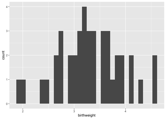
Setting the “binwidth” parameter within the geom_histogram() call changes the appearance of the plot and eliminates the message.
ggplot(data = experiment, mapping = aes(x = birthweight)) +
  geom_histogram(binwidth = 1)
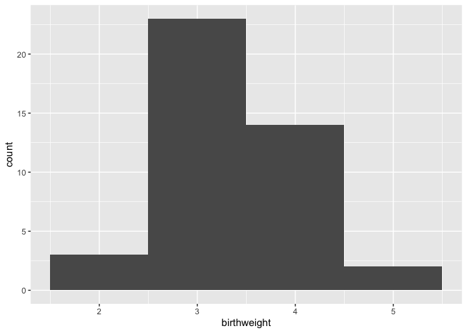
ggplot(data = experiment, mapping = aes(x = birthweight)) +
  geom_histogram(binwidth = 0.25)
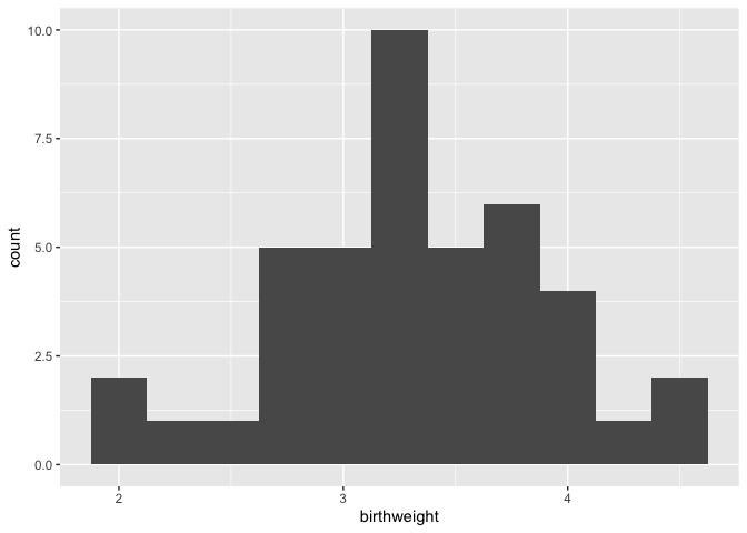
Adding color (and fill) to geoms
The color (for lines and points) and fill (for areas, like bars) of a geom can add another layer of information to the plot.
ggplot(data = experiment, mapping = aes(x = birthweight, fill = location)) +
  geom_histogram(binwidth = 0.25) +
  scale_fill_manual(values = locations.palette)
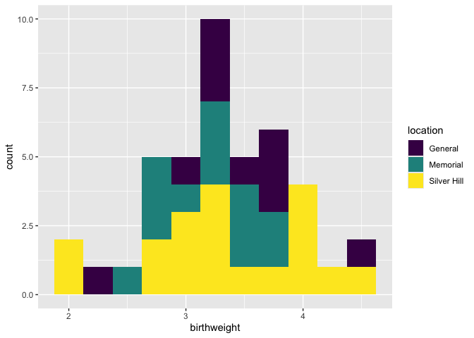
Here the total height of the bar is equal to the number of births at each weight, and the fill denotes the hospital at which the birth occurred.
ggplot(data = experiment, mapping = aes(x = birthweight, fill = location)) +
  geom_histogram(binwidth = 0.25, position = position_dodge()) +
  scale_fill_manual(values = locations.palette)
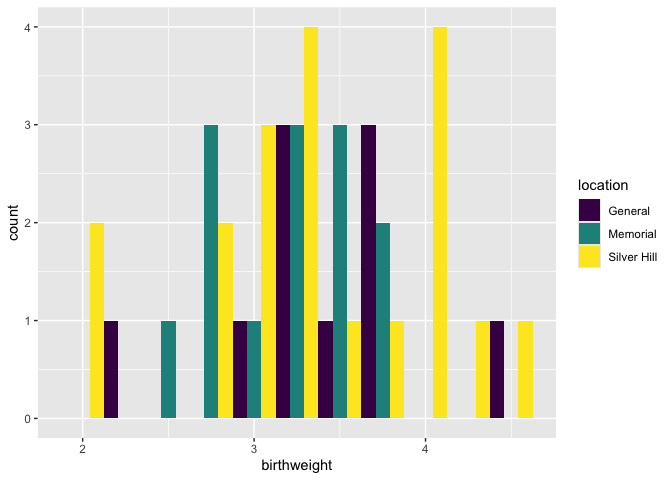
To un-stack the bars, use “position_dodge.”
Creating faceted plots
Sometimes, it may be more clear graphically to create multiple sub-plots or “facets” based on categorical values in the data. The facet_wrap() and facet_grid() functions allow the user to break the data down into multiple plots by one or two categorical variables, respectively.
ggplot(data = experiment, mapping = aes(x = birthweight, fill = location)) +
  geom_histogram(binwidth = 0.25) +
  scale_fill_manual(values = locations.palette) +
  facet_wrap(~year, nrow = 2)
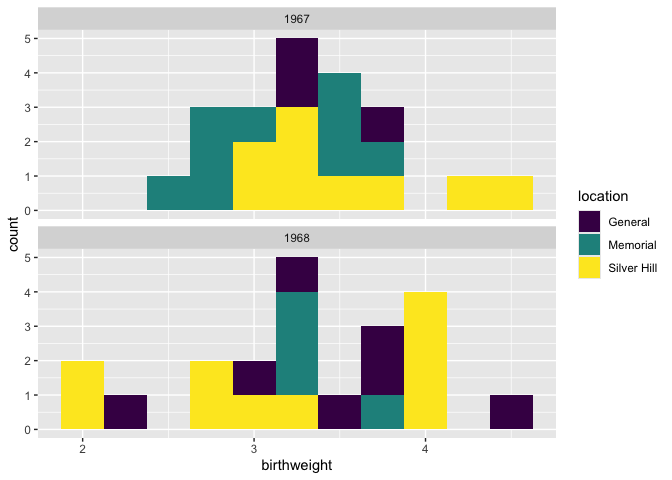
Add and modify labels
Often, the aesthetic names (column names) are uninformative, or unattractive. This may not make much difference when making exploratory figures, but in a report or publication, it is important to have a greater degree of control over the plot title, axis labels, and so on. The labs() function offers the option to set the following labels:
- any aesthetic that has been set: in this case, x and fill
- title: main title of the plot
- subtitle: displayed below the title
- caption: displayed at the bottom right of the plot by default
- tag: label that appears at the top left of the plot by default (e.g. 1A)
- alt, alt_insight: alt text for the plot (used by screen readers)
ggplot(data = experiment, mapping = aes(x = birthweight, fill = location)) +
  geom_histogram(binwidth = 0.25) +
  scale_fill_manual(values = locations.palette) +
  facet_wrap(~year, nrow = 2) +
  labs(x = "birth weight (kg)",
       fill = "Hospital",
       tag = "fig. 1",
       caption = "Birth weights by year, color-coded by delivery location.",
       alt = "Pair of histograms displaying the distribution of birth weights of infants born at General Hospital, Memorial Hospital, and Silver Hill Medical Center in 1967 and 1968.")
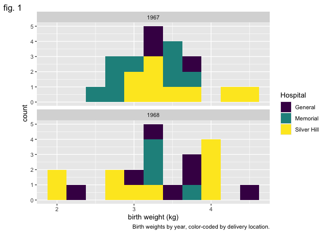
Making global changes to the plot’s appearance using themes
The “theme” of a ggplot object controls the graphical elements that are not mapped onto the data. This includes things like the font size and alignment of axis labels and the color of the plot background. There are a number of pre-set themes offering a range of plot styles.
In addition, the theme() function offers access to these graphical elements independently. Using it, you can change the angle of the text on the x axis, the placement of the legend, and many other things. Here, we will use it to remove the legend title.
ggplot(data = experiment, mapping = aes(x = birthweight, fill = location)) +
  geom_histogram(binwidth = 0.25) +
  scale_fill_manual(values = locations.palette) +
  facet_grid(location~year) +
  labs(x = "weight (kg)", y = "births") +
  theme_bw() +
  theme(legend.title = element_blank())
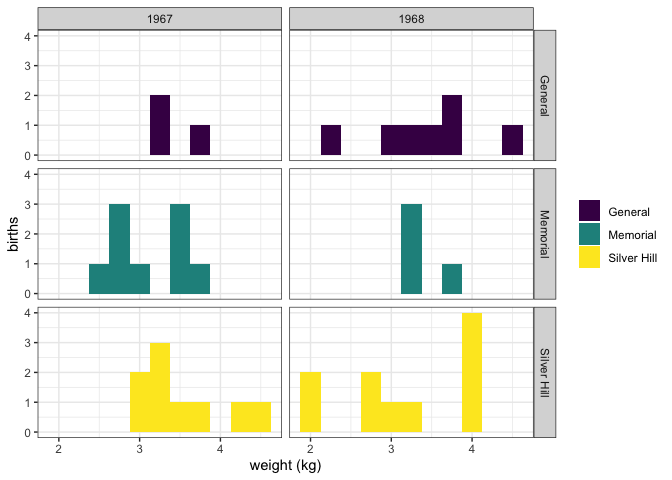
An interesting alternative to geom_histogram() is geom_density().
ggplot(data = experiment, mapping = aes(x = birthweight, fill = smoker)) +
  geom_density(alpha = 0.5) +
  scale_fill_manual(values = smoking.palette) +
  labs(x = "birth weight (kg)", fill = "Maternal smoking in pregnancy") +
  theme_bw()
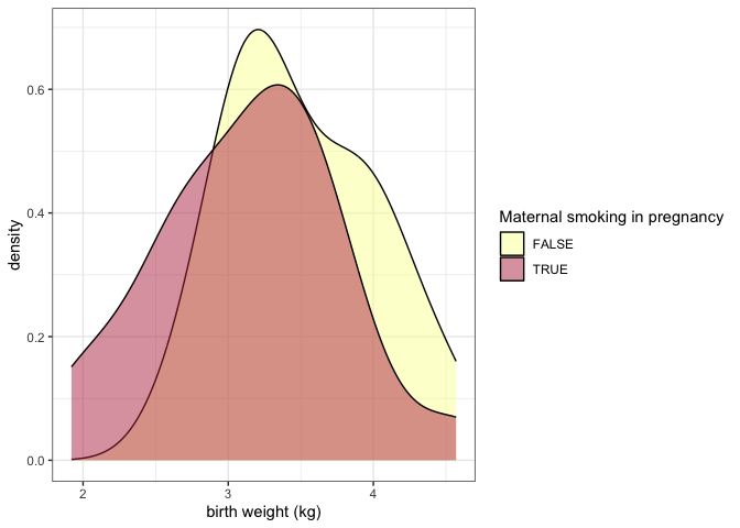
The alpha channel of a color determines its opacity. In this case, we have placed alpha = 0.5 outside of the aes() function call, because the opacity is not being mapped to any characteristic of the data.
The examples above use color in a discrete fashion. In the scatter plot below, the color of each point represents a birth weight (continuous variable).
experiment %>%
  filter(smoker == TRUE) %>%
  ggplot(mapping = aes(x = maternal.cigarettes,
                       y = weeks.gestation,
                       color = birthweight)) +
  geom_point()  +
  labs(x = "Maternal cigarettes / day", y = "Gestational age at birth (weeks)", color = "Birth weight (kg)") +
  scale_color_viridis(option = "inferno", begin = 0.4) +
  theme_bw()
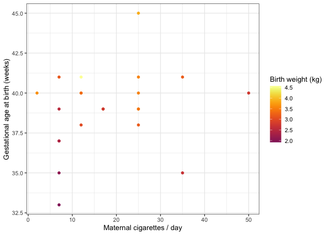
Notice that it is not necessary to specify a color palette; viridis has a built-in function for interacting with ggplot objects.
Change the labels for categorical values
All of the elements of the plot, not just the height of bars and position of points, convey information. The labels on a categorical axis should be meaningful.
experiment %>%
  ggplot(mapping = aes(x = smoker, y = birthweight, fill = smoker)) +
  geom_boxplot() +
  scale_fill_manual(values = smoking.palette) +
  theme_bw()
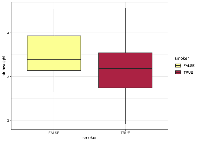
The bar chart above displays the values “TRUE” and “FALSE” on the x-axis. This is fine for an exploratory plot, but in a report or publication, it might be more informative to replace them with “smoker” and “non-smoker.” The scale_x_discrete() function allows us to do just that.
experiment %>%
  ggplot(mapping = aes(x = smoker, y = birthweight, fill = smoker)) +
  geom_boxplot() +
  scale_fill_manual(values = smoking.palette) +
  scale_x_discrete(labels = c("non-smoker", "smoker")) +
  guides(fill = "none") +
  labs(y = "birth weight (kg)", x = "maternal cigarette use in pregnancy") +
  theme_bw()
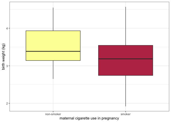
Change the direction of axes to improve readability
If the category names are very long, it may be necessary to change the direction of the axis labels.
experiment %>%
  ggplot(mapping = aes(x = smoker, y = birthweight, fill = smoker)) +
  geom_boxplot() +
  scale_fill_manual(values = smoking.palette) +
  scale_x_discrete(labels = c("non-smoking in pregnancy", "cigarette smoking in pregnancy")) +
  guides(fill = "none") +
  labs(y = "birth weight (kg)") +
  theme_bw() +
  theme(axis.title.x = element_blank(),
        axis.text.x = element_text(angle = 90, vjust = 0.5, hjust = 1))
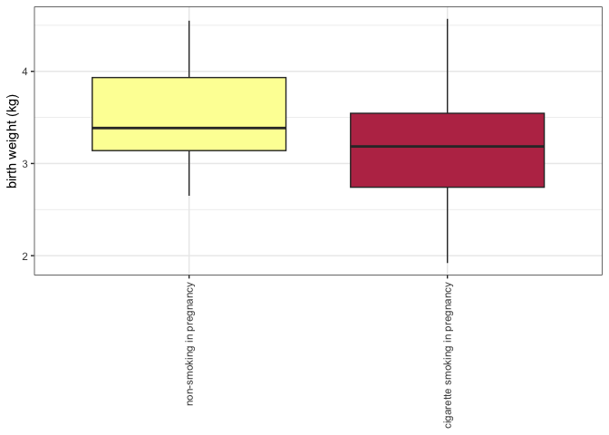
Or even the direction of the axes themselves.
experiment %>%
  ggplot(mapping = aes(x = smoker, y = birthweight, fill = smoker)) +
  geom_boxplot() +
  scale_fill_manual(values = smoking.palette) +
  scale_x_discrete(labels = c("non-smoking in pregnancy", "cigarette smoking in pregnancy")) +
  guides(fill = "none") +
  labs(y = "birth weight (kg)") +
  coord_flip() +
  theme_bw() +
  theme(axis.title.y = element_blank())
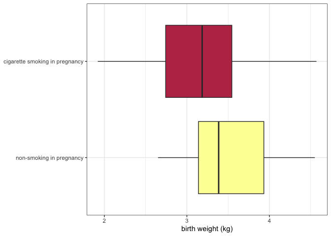
The pivot_longer() function revisited
In the previous section on Tidyverse, pivot_longer() was only briefly discussed. This is because the easiest way to explain why it is useful is to demonstrate.
experiment %>%
  pivot_longer(cols = c(22:25),
               names_to = "gene.id",
               values_to = "expression") %>%
  ggplot(mapping = aes(x = smoker, y = expression, fill = smoker)) +
  geom_violin() +
  scale_fill_manual(values = smoking.palette) +
  scale_x_discrete(labels = c("non-smoker", "smoker")) +
  facet_wrap(~ gene.id, nrow = 2) +
  guides(fill = "none") +
  labs(x = "Maternal tobacco use in pregnancy", y = "miRNA expression") +
  theme_bw()
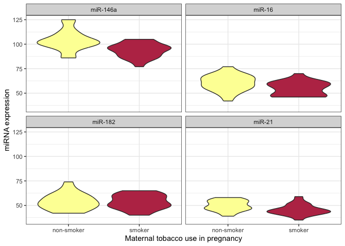
After pivoting the miRNA data into a single column called expression, that data is available for ggplot to map that onto an aesthetic property.
Use shape and line type to convey meaning
Color is not the only aesthetic available for mapping to the data. Shape and line type are also good candidates for displaying categorical (or discrete) values.
experiment %>%
  pivot_longer(cols = c(22:25),
               names_to = "gene.id",
               values_to = "expression") %>%
  ggplot(mapping = aes(x = maternal.cigarettes, y = expression, color = location, shape = low.birthweight)) +
  geom_point() +
  scale_color_manual(values = locations.palette) +
  scale_shape_manual(values = c(16, 17), labels = c("< 2.72 kg", ">= 2.72 kg")) +
  facet_wrap(~ gene.id, nrow = 2) +
  labs(x = "Maternal cigarettes / day", y = "miRNA expression") +
  theme_bw() +
  theme(legend.title = element_blank())
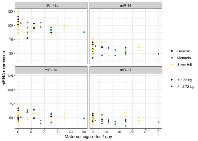
There are 25 shapes available for plotting. You can see them all here.
experiment %>%
  ggplot(mapping = aes(x = weeks.gestation, y = birthweight, linetype = smoker)) +
  geom_quantile(quantiles = c(0.25, 0.5, 0.75), color = "black") +
  labs(x = "gestational age at birth", y = "birth weight (kg)", linetype = "geriatric preganancy") +
  theme_bw()
## Smoothing formula not specified. Using: y ~ x
## Smoothing formula not specified. Using: y ~ x
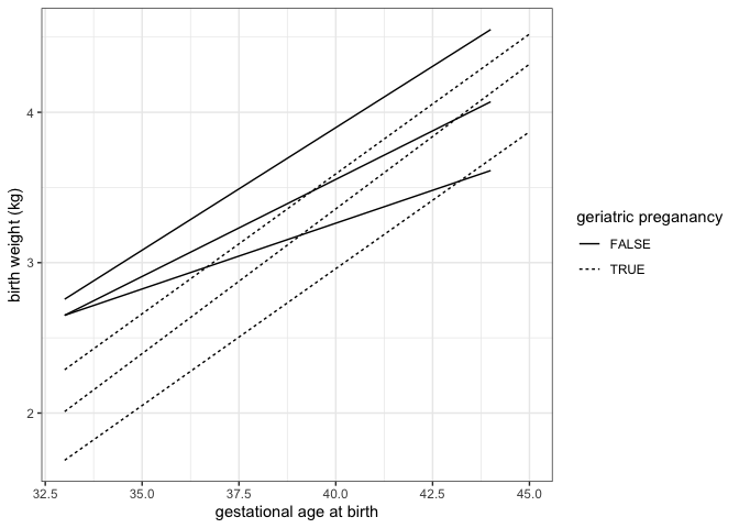
Focus in on one portion of the plot
We can zoom in to the the lower left hand corner of the plot using coord_cartesian().
experiment %>%
  ggplot(mapping = aes(x = weeks.gestation, y = birthweight, linetype = smoker)) +
  geom_quantile(quantiles = c(0.25, 0.5, 0.75), color = "black") +
  labs(x = "gestational age at birth", y = "birth weight (kg)", linetype = "geriatric preganancy") +
  coord_cartesian(xlim = c(33, 35), ylim = c(1.5, 3.5)) +
  theme_bw()
## Smoothing formula not specified. Using: y ~ x
## Smoothing formula not specified. Using: y ~ x
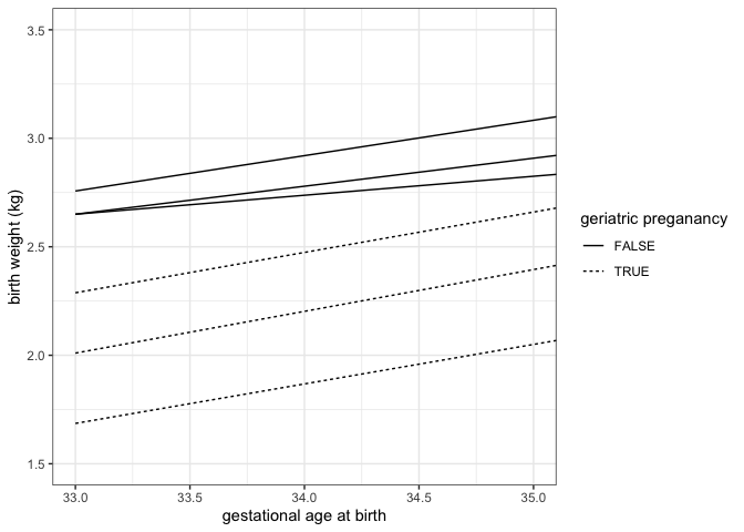
Layer multiple geoms
It is not necessary to make a single geom convey all of the information a plot must communicate. Instead, ggplot2 offers users the ability to layer geoms together. As long as they use the same axes, geoms may share a plot.
ggplot(experiment, mapping = aes(x = weeks.gestation,
                                 y = birthweight,
                                 color = smoker)) +
  geom_point() +
  geom_smooth(alpha = 0.2) +
  labs(x = "Gestational age at birth (weeks)",
       y = "Birth weight (kg)",
       color = "Maternal tobacco use",
       caption = "Birthweight increases with gestational age for infants born to both\nsmokers and non-smokers.") +
  scale_color_manual(values = smoking.palette) +
  theme_bw() +
  theme(plot.caption = element_text(hjust = 0))
## `geom_smooth()` using method = 'loess' and formula = 'y ~ x'
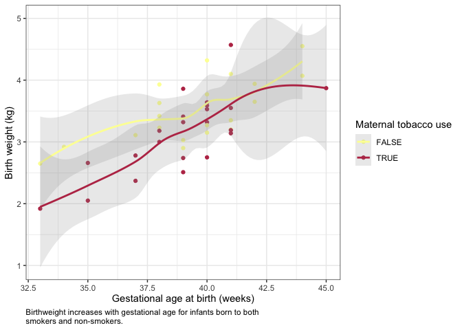
experiment %>%
  group_by(year, smoker) %>%
  summarise(mean.birthweight = mean(birthweight),
            sd.birthweight = sd(birthweight)) %>%
  ggplot(mapping = aes(x = as.factor(year), y = mean.birthweight, fill = smoker)) +
  geom_col(position = position_dodge2(preserve = "single")) +
  geom_errorbar(mapping = aes(ymin = mean.birthweight - sd.birthweight,
                              ymax = mean.birthweight + sd.birthweight),
                position = position_dodge2(preserve = "single")) +
  scale_fill_manual(values = smoking.palette) +
  labs(x = "birth year", y = "birth weight (kg)", fill = "maternal smoking") +
  theme_bw()
## `summarise()` has grouped output by 'year'. You can override using the
## `.groups` argument.
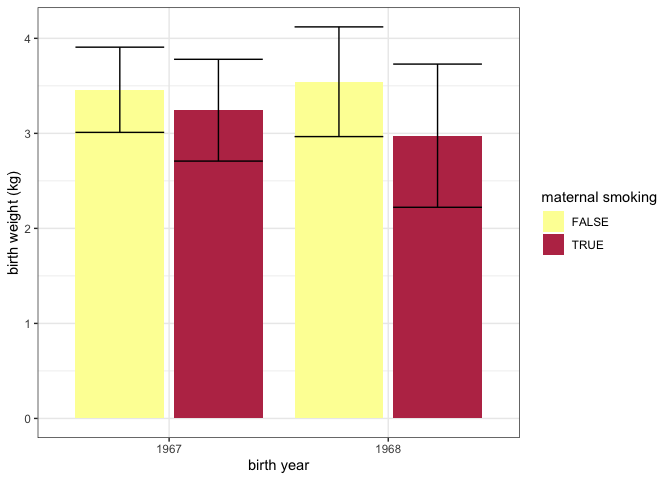
ggplot2 cheat sheet
For more information on ggplot2 check out this quick reference guide, and the free online book.
Exercise 5
Create a visualization that provides an answer to one of the following questions:
- Are preterm babies more likely to have low birth weight?
- What is the ratio of maternal cigarettes to paternal cigarettes for births at each of the hospitals?
- Do taller mothers have taller partners? Do they have longer babies?
Troubleshooting
Even advanced users of R run into problems often. Here are some of the most common errors that can often be resolved quickly:
- file is not in the right place, or is incorrectly named
- improperly formatted files
- missing values
- spelling errors
- incorrectly named parameters
For more complex errors, the help documentation of a function is a good place to start. Additionally, the online community of R users is extremely active and helpful. If you’ve got a question, it’s extremely likely it’s been asked and answered many times already!