
Introduction to Python
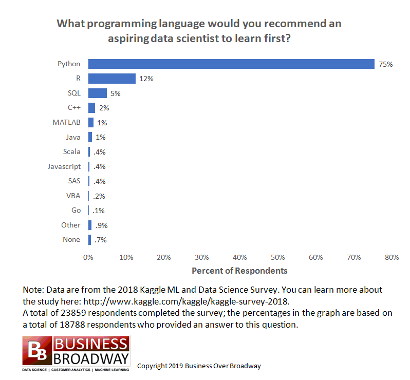
Why Python
https://businessoverbroadway.com/2019/01/13/programming-languages-most-used-and-recommended-by-data-scientists/
https://www.tiobe.com/tiobe-index/
- Python is extremely popular and widely used, especially for data science.
- Popular and getting more so in Bioinformatics, especially for building tools.
- For analysis, R is arguably more useful currently due to the huge number of packages available from Bioconductor and CRAN.
- The best option is to learn Python, R, and bash. A little of each will go a long way.
- Freely available to download for Windows, Linux, Mac OS X, etc.
- Python is extremely versatile
- Used for a wide range of purposes from automating simple tasks to massive software projects with wide adoption by many large companies.
- Installed on almost every Linux server.
- Vast number of resources online: If you can Google for it you can learn how to do it.
Background
What is a programming language and why do we need it?
Speaking to a computer in its native language is tedious and complicated. A programming language is a way for humans to describe a set of operations to a computer in a more abstract and understandable way. A helper program then translates our description of the operations into a set of instructions (machine code) for the computer to carry out.
Some day we may develop a programming language that allows us to communicate our instructions to the computer in our native language (Alexa, turn on the TV). Except for simple cases, this option doesn’t exist yet, largely because human languages are complicated and instructions can be difficult to understand (even for other humans).
In order for the helper program to work properly, we need to use a concise language:
- Well defined vocabulary for describing the basic set of supported operations.
- Well defined set of Data Types that have a defined set of valid operations (add, subtract, etc).
- Well defined syntax that leaves no ambiguity about when the computer should carry out each instruction.
Specifically in Python:
A brief history of Python
- Initially developed during the late 1980’s by Guido van Rossum, BDFL until 2018.
- First development version released in 1991. Version 1 released in 1994.
- Python 2.0.0 released June, 2001
- Python 2.x end-of-life Jan 1, 2020.
- This version was so popular and widely used that many Bioinformatics programs were written using it. Some of these tools have been converted to support v3.x, others are in the process of being upgraded or have been abandoned and will stay on v2.x. The last Python 2.x release is still available for download.
- Python 3.x (December 2008) was a significant re-design and broke compatibility with some parts of v2.x.
- The current version is 3.14.
Interesting features of Python
- High level: It hides a lot of the complicated details.
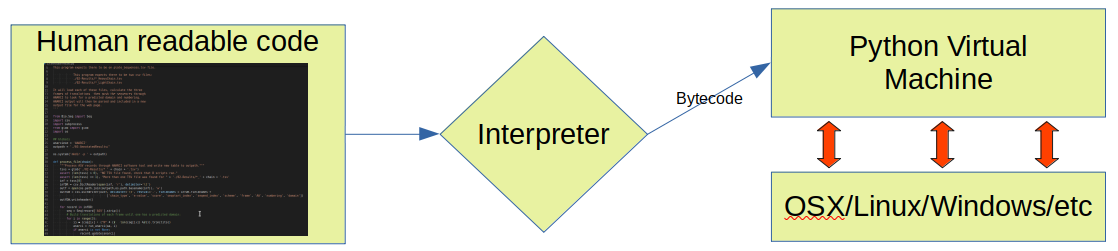
- Interpreted: programs are compiled to byte code and run on a virtual machine instead of being compiled to native machine language
- This provides the option of running Python interactively, or writing Python scripts.
- Garbage Collected: memory is allocated and freed for you automatically
- Spaces matter in Python and are part of the language syntax. Be careful with copy/paste!
- In Python, “Readability counts”.
- There is a style guide called Python Enhancement Proposal 8 (PEP8) that documents and encourages consistent, readable code. If you plan to share your code with others, it is good practice to follow the style guide (or adopt the style used by the rest of the team).
- These best practices are also known as writing “pythonic” or “idiomatic” python, this guide has more details. Try
import thisin your Python interpreter if you are a fan of programmer philosophy.
Base Python and the extensive package ecosystem
- Python has been extremely successful partly because it is modular and highly extensible. The core of Python is relatively small and compact, but this is supplemented with a large “standard library” that adds a large amount of additional functionality.
- Thousands of additional packages are available from the PyPI repository.
- PythonPath variable
- Where do libraries live?
- Virtual Environments
- Conflicts and package versions
- Virtual environments
- Conda
Project Jupyter
- Developed for interactive data science and scientific computing across all programming languages
- Non-profit, open-source
- Free
Disclaimer
Learning all the nuances of python takes a long time! Our goal here is to introduce you to as many concepts as possible but if you are serious about mastering python you will need to apply yourself beyond this introduction.
Installation
We are going to use a python distribution platform, Anaconda. It was designed to meet the demand of Data Sciences and AI projects. It can be installed on all three operating systems and has 45 million users as of 2024. It includes over 300 packages, offers jupyter Notebooks and jupyter Lab and includes conda, the package and environment manager. It makes installing a lot of python packages very easy. Please follow the instructions below to install Anaconda. Instructions for all platforms can be found at https://www.anaconda.com/docs/getting-started/anaconda/install
- Macs: Two options are available. One is to use the graphic installer. The other is to use the Command Line installer.
- For graphic installer, please go to https://www.anaconda.com/download and follow the instructions in the “Download Now” panel. This option installs Anaconda in /opt/anacondas in the file system. In order to install Anaconda into your Home directory (especially in the case where there are multiple users), Command Line installation is recommended.
- For Command Line installer
- Mac Arm64 architecture
- Download: wget https://repo.anaconda.com/archive/Anaconda3-2025.06-0-MacOSX-arm64.sh
- Install: bash Anaconda3-2025.06-0-MacOSX-arm64.sh
- Mac Intel architecture
- Download: wget https://repo.anaconda.com/archive/Anaconda3-2025.06-0-MacOSX-x86_64.sh
- Install: bash Anaconda3-2025.06-0-MacOSX-x86_64.sh
- Mac Arm64 architecture
- Linux:
- Download: wget https://repo.anaconda.com/archive/Anaconda3-2025.06-0-Linux-x86_64.sh
- Install: bash Anaconda3-2025.06-0-Linux-x86_64.sh
- Windows: Please install in your ubuntu subsystem so that conda is available for installing other python packages later
- Download: wget https://repo.anaconda.com/archive/Anaconda3-2025.06-0-Linux-x86_64.sh
- Install: bash Anaconda3-2025.06-0-Linux-x86_64.sh
After Anaconda is successfully installed, please open a new Command Line interface to be able to use the installed libraries. If you have chosen to ask the installer not to add configuration to your initialize conda every time you open a new shell, you will have to do it manualy when you need to access any program that Anaconda has installed. Using the following commands in the new Command Line window will accomplish this task.
source <PATH_TO_CONDA>/bin/activate
conda init –all
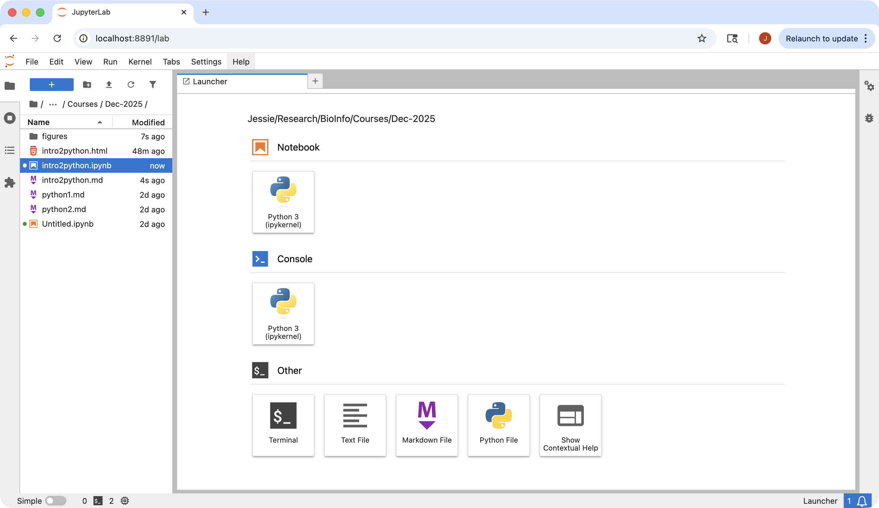
The way to launch a jupyter lab session in command line is to use the following command.
Once this command is run, you will see a message similar to the following to provide urls for your web browser to start the interactive session.
To access the server, open this file in a browser:
    file:///Users/jli/Library/Jupyter/runtime/jpserver-86015-open.html
Or copy and paste one of these URLs:
    http://localhost:8892/lab?token=99e0c0136bcee32edfc8ce37c673f5dc1940bb2a307fc3d3
    http://127.0.0.1:8892/lab?token=99e0c0136bcee32edfc8ce37c673f5dc1940bb2a307fc3d3
Hello World!
[Input:]
print("Hello World!")
[Output:]
Hello World!
Functions and how to find help
As in any other programming language, a function is a predefined set of operations. In order to find the information on what parameters a function requires, one has 2 options:
- use the help() function
- use shift + tab
[Input:]
help(print)
[Output:]
Help on built-in function print in module builtins:

print(*args, sep=' ', end='\n', file=None, flush=False)
    Prints the values to a stream, or to sys.stdout by default.

    sep
      string inserted between values, default a space.
    end
      string appended after the last value, default a newline.
    file
      a file-like object (stream); defaults to the current sys.stdout.
    flush
      whether to forcibly flush the stream.
*args means that the function print can accept any number of arguments.
Basic Data Types
Built in data types
| Data type | Functions |
|---|---|
| Text/Character | str() |
| Numeric | int(), float(), complex() |
| Sequence | list()/[], tuple()/(), range() |
| Mapping | dict()/{} |
| Set | set()/{}, frozenset() |
| Boolean | bool() |
| Binary | bytes(), bytearray(), memoryview() |
| None | None |
Integers, Floating-point numbers, booleans, strings.
| Language | Python | R |
|---|---|---|
| Integer data | int() | as.integer(), integer() |
| Float data | float() | numeric() |
| Logical data | bool(), [True, False] | as.logical(), logical(), (TRUE, FALSE) |
| Character data | str() | as.character(), character() |
Integer
[Input:]
a = int(5)
[Input:]
a
[Output:]
5
[Input:]
b = 5
[Input:]
b
[Output:]
5
[Input:]
type(a)
[Output:]
int
[Input:]
type(b)
[Output:]
int
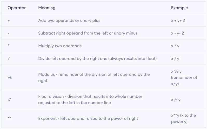
Arithmetic operators
Exercise
Creat different data types (integers, floats, booleans and strings) and perform some operations.
Sequence data
| Data type | Usage | Characteristics |
|---|---|---|
| Lists | Store multiple items in a single variable | Ordered, mutable, allow duplicate values |
| Tuples | Store multiple items in a single variable | Ordered, immutable, allow duplicate values |
| Range | Create an immutable sequence of numbers | Immutable, a range of integers |
Immutable means that an object’s state or value cannot be changed after its creation. Let’s take a look at one example to understand what immutable means in python. Here we will create a variable using range() function.
Range
[Input:]
range_example = range(6)
[Input:]
range_example
[Output:]
range(0, 6)
[Input:]
range_example[0]
[Output:]
0
[Input:]
range_example[0] = 3
[Output:]
Error:
---------------------------------------------------------------------------
TypeError                                 Traceback (most recent call last)
Cell In[12], line 1
----> 1 range_example[0] = 3

TypeError: 'range' object does not support item assignment
[Input:]
range_example[5]
[Output:]
5
[Input:]
range_example[6] = 8
[Output:]
Error:
---------------------------------------------------------------------------
TypeError                                 Traceback (most recent call last)
Cell In[14], line 1
----> 1 range_example[6] = 8

TypeError: 'range' object does not support item assignment
Range function is usually used in a for loop. For example,
[Input:]
protein_seq = "MTKAAVGLVKNRAWGIPSDF"
protein_len = len(protein_seq)
for i in range(protein_len):
    print("The ", i+1, "th amino acid is: ", protein_seq[i])
[Output:]
The  1 th amino acid is:  M
The  2 th amino acid is:  T
The  3 th amino acid is:  K
The  4 th amino acid is:  A
The  5 th amino acid is:  A
The  6 th amino acid is:  V
The  7 th amino acid is:  G
The  8 th amino acid is:  L
The  9 th amino acid is:  V
The  10 th amino acid is:  K
The  11 th amino acid is:  N
The  12 th amino acid is:  R
The  13 th amino acid is:  A
The  14 th amino acid is:  W
The  15 th amino acid is:  G
The  16 th amino acid is:  I
The  17 th amino acid is:  P
The  18 th amino acid is:  S
The  19 th amino acid is:  D
The  20 th amino acid is:  F
List
A list can be created by using the function list() and by using [].
[Input:]
list_example = ["NDUFAF7", "AGMAT", "TOP1MT", "IARS2", "MTFP1", "SLC25A51", "PRORP", "SLC25A52", "ENDOG"]
[Input:]
list_example
[Output:]
['NDUFAF7',
 'AGMAT',
 'TOP1MT',
 'IARS2',
 'MTFP1',
 'SLC25A51',
 'PRORP',
 'SLC25A52',
 'ENDOG']
[Input:]
len(list_example)
[Output:]
9
[Input:]
type(list_example)
[Output:]
list
List is mutable, which means that one may modify the values of a list after its creation.
| Function | Operation |
|---|---|
| append | Add an element at the end of the list |
| extend | Add multiple elements at the end of the list |
| insert | Add an element at a specific position |
| remove | Remove the first occurrence of an element |
| pop | Removes an element at a specific position or the last element if no index is specified |
| del | Delete object |
For example, let’s add an element to list_example
[Input:]
list_example.append("CKMT2")
list_example
[Output:]
['NDUFAF7',
 'AGMAT',
 'TOP1MT',
 'IARS2',
 'MTFP1',
 'SLC25A51',
 'PRORP',
 'SLC25A52',
 'ENDOG',
 'CKMT2']
We see a new syntax, object.function(). This is the way to call a method that is bound to an object in python. A method is a function that is defined specifically for an object of a class in python. In order to know what methods are bound to an object, we can use the following operation:
- methods = [method_name for method_name in dir(obj) if callable(getattr(obj, method_name)) and not method_name.startswith(“__”)]
[Input:]
methods = [method_name for method_name in dir(list_example) if callable(getattr(list_example, method_name)) and not method_name.startswith("__")]
methods
[Output:]
['append',
 'clear',
 'copy',
 'count',
 'extend',
 'index',
 'insert',
 'pop',
 'remove',
 'reverse',
 'sort']
Exercise
Let’s modify list_example by using the functions listed above, add element(s), delete element(s), …
Mapping data - Dictionaries
Dictionaries in python store data in key:value pairs.
- An ordered collection (starting in python 3.7)
- Changable
- Do not allow duplicate keys
- Allows for fast key lookup
- Values can be any python data type
Syntax:
{
Key1: value1,
Key2: value2,
…,
KeyN: valueN,
}
[Input:]
dict_example = {
    "gene_name": "CKMT2",
    "gene_biotype": "protein_coding",
    "n_transcripts": 32,
    "n_orthologues": 217,
    "n_paralogues": 4,
    "ensembl_id": "ENSG00000131730",
    "discription": "creatine kinase, mitochondrial 2",
    "loc": "Chromosome 5: 81,233,320-81,266,399",
    "strand": "+",}
dict_example
[Output:]
{'gene_name': 'CKMT2',
 'gene_biotype': 'protein_coding',
 'n_transcripts': 32,
 'n_orthologues': 217,
 'n_paralogues': 4,
 'ensembl_id': 'ENSG00000131730',
 'discription': 'creatine kinase, mitochondrial 2',
 'loc': 'Chromosome 5: 81,233,320-81,266,399',
 'strand': '+'}
Access items in the dictionary
- The most intuitive way is to use the keys.
[Input:]
dict_example["gene_name"]
[Output:]
'CKMT2'
But how do one know what keys there are in a dictionary object?
[Input:]
methods = [method_name for method_name in dir(dict_example) if callable(getattr(dict_example, method_name))
           and not method_name.startswith("__")]
methods
[Output:]
['clear',
 'copy',
 'fromkeys',
 'get',
 'items',
 'keys',
 'pop',
 'popitem',
 'setdefault',
 'update',
 'values']
[Input:]
dict_example.keys()
[Output:]
dict_keys(['gene_name', 'gene_biotype', 'n_transcripts', 'n_orthologues', 'n_paralogues', 'ensembl_id', 'discription', 'loc', 'strand'])
How does one extract the values of more than one key. For example, let’s try to extract values of some keys, gene_name, gene_biotype, and n_transcripts. This can be done easily using a for loop.
[Input:]
for key in ["gene_name", "gene_biotype", "n_transcripts"]:
    print(f"{key}: ", dict_example.get(key))
[Output:]
gene_name:  CKMT2
gene_biotype:  protein_coding
n_transcripts:  32
In another example, we are going to update the dictionary with an additional piece of information, using the method update.
[Input:]
dict_example.update({"pathway": "Mitochondria disease pathway"})
dict_example
dict_example.update(pathway_members = 10)
dict_example
[Output:]
{'gene_name': 'CKMT2',
 'gene_biotype': 'protein_coding',
 'n_transcripts': 32,
 'n_orthologues': 217,
 'n_paralogues': 4,
 'ensembl_id': 'ENSG00000131730',
 'discription': 'creatine kinase, mitochondrial 2',
 'loc': 'Chromosome 5: 81,233,320-81,266,399',
 'strand': '+',
 'pathway': 'Mitochondria disease pathway',
 'pathway_members': 10}
Because the values can be any python data type, one may create nested dictionaries.
[Input:]
nested_dict = {
    "ENSG00000131730": {
        "gene_name": "CKMT2",
        "gene_biotype": "protein_coding",
        "n_transcripts": 32,
        "n_orthologues": 217,
        "n_paralogues": 4,
        "ensembl_id": "ENSG00000131730",
        "discription": "creatine kinase, mitochondrial 2",
        "loc": "Chromosome 5: 81,233,320-81,266,399",
        "strand": "+",},
    "ENSG00000003509": {
        "gene_name": "NDUFAF7",
        "gene_biotype": "protein_coding",
        "n_transcripts": 20,
        "n_orthologues": 210,
        "n_paralogues": 0,
        "ensembl_id": "ENSG00000003509",
        "discription": "NADH:ubiquinone oxidoreductase complex assembly factor 7",
        "loc": "Chromosome 2: 37,231,631-37,253,403 ",
        "strand": "+",},
}
[Input:]
nested_dict
[Output:]
{'ENSG00000131730': {'gene_name': 'CKMT2',
  'gene_biotype': 'protein_coding',
  'n_transcripts': 32,
  'n_orthologues': 217,
  'n_paralogues': 4,
  'ensembl_id': 'ENSG00000131730',
  'discription': 'creatine kinase, mitochondrial 2',
  'loc': 'Chromosome 5: 81,233,320-81,266,399',
  'strand': '+'},
 'ENSG00000003509': {'gene_name': 'NDUFAF7',
  'gene_biotype': 'protein_coding',
  'n_transcripts': 20,
  'n_orthologues': 210,
  'n_paralogues': 0,
  'ensembl_id': 'ENSG00000003509',
  'discription': 'NADH:ubiquinone oxidoreductase complex assembly factor 7',
  'loc': 'Chromosome 2: 37,231,631-37,253,403 ',
  'strand': '+'}}
[Input:]
nested_dict["ENSG00000131730"]["discription"]
[Output:]
'creatine kinase, mitochondrial 2'
Keys() function can be used to list all the keys in a dictionary.
[Input:]
nested_dict.keys()
[Output:]
dict_keys(['ENSG00000131730', 'ENSG00000003509'])
[Input:]
nested_dict['ENSG00000131730'].keys()
[Output:]
dict_keys(['gene_name', 'gene_biotype', 'n_transcripts', 'n_orthologues', 'n_paralogues', 'ensembl_id', 'discription', 'loc', 'strand'])
Dictionaries can be created using dict() function.
[Input:]
gene_names = ["CKMT2", "NDUFAF7", "AGMAT"]
gene_biotypes = ["protein_coding"] * 3
n_transcripts = [32, 20, 4]
n_orthologues = [217, 210, 195]
n_paralogues = [4, 0, 2]
ensembl_IDs = ["ENSG00000131730", "ENSG00000003509", "ENSG00000116771"]
descriptions = ["creatine kinase, mitochondrial 2", "NADH:ubiquinone oxidoreductase complex assembly factor 7",
                "agmatinase (putative)"]
locus = ["Chromosome 5: 81,233,320-81,266,399", "Chromosome 2: 37,231,631-37,253,403", "Chromosome 1: 15,571,699-15,585,078"]
strands = ["+", "+", "-"]
list_values = zip(gene_names, gene_biotypes, n_transcripts, n_orthologues,
                  n_paralogues, ensembl_IDs, descriptions, locus, strands)
list_keys = ["gene_name", "gene_biotype", "n_transcripts", "n_orthologues",
             "n_paralogues", "ensembl_ID", "Description", "loc", "strand"]
list_dict = [dict(zip(list_keys, value)) for value in list_values]
list_dict
[Output:]
[{'gene_name': 'CKMT2',
  'gene_biotype': 'protein_coding',
  'n_transcripts': 32,
  'n_orthologues': 217,
  'n_paralogues': 4,
  'ensembl_ID': 'ENSG00000131730',
  'Description': 'creatine kinase, mitochondrial 2',
  'loc': 'Chromosome 5: 81,233,320-81,266,399',
  'strand': '+'},
 {'gene_name': 'NDUFAF7',
  'gene_biotype': 'protein_coding',
  'n_transcripts': 20,
  'n_orthologues': 210,
  'n_paralogues': 0,
  'ensembl_ID': 'ENSG00000003509',
  'Description': 'NADH:ubiquinone oxidoreductase complex assembly factor 7',
  'loc': 'Chromosome 2: 37,231,631-37,253,403',
  'strand': '+'},
 {'gene_name': 'AGMAT',
  'gene_biotype': 'protein_coding',
  'n_transcripts': 4,
  'n_orthologues': 195,
  'n_paralogues': 2,
  'ensembl_ID': 'ENSG00000116771',
  'Description': 'agmatinase (putative)',
  'loc': 'Chromosome 1: 15,571,699-15,585,078',
  'strand': '-'}]
Exercise
Please apply the methods available for a dictionary object to get familiar with this data type.
List comprehension
List comprehension is a very useful method available in python. It creates a new list by performing a pre-defined set of operations on each element of an existing list.
- Short syntax for better readability
- Faster operation than a for loop
- Creates a new list
New_list = [expression for item in iterable if condition == True]
[Input:]
list_values = zip(gene_names, gene_biotypes, n_transcripts, n_orthologues,
                  n_paralogues, ensembl_IDs, descriptions, locus, strands)
list_dict = [dict(zip(list_keys, value)) for value in list_values]
list_dict
[Output:]
[{'gene_name': 'CKMT2',
  'gene_biotype': 'protein_coding',
  'n_transcripts': 32,
  'n_orthologues': 217,
  'n_paralogues': 4,
  'ensembl_ID': 'ENSG00000131730',
  'Description': 'creatine kinase, mitochondrial 2',
  'loc': 'Chromosome 5: 81,233,320-81,266,399',
  'strand': '+'},
 {'gene_name': 'NDUFAF7',
  'gene_biotype': 'protein_coding',
  'n_transcripts': 20,
  'n_orthologues': 210,
  'n_paralogues': 0,
  'ensembl_ID': 'ENSG00000003509',
  'Description': 'NADH:ubiquinone oxidoreductase complex assembly factor 7',
  'loc': 'Chromosome 2: 37,231,631-37,253,403',
  'strand': '+'},
 {'gene_name': 'AGMAT',
  'gene_biotype': 'protein_coding',
  'n_transcripts': 4,
  'n_orthologues': 195,
  'n_paralogues': 2,
  'ensembl_ID': 'ENSG00000116771',
  'Description': 'agmatinase (putative)',
  'loc': 'Chromosome 1: 15,571,699-15,585,078',
  'strand': '-'}]
Let’s dissect the operation
[dict(zip(list_keys, value)) for value in list_values]
Exercise
Create a numeric iterable object and perform the same operation on each element of the object without using a for loop.
Challenge
- What is the difference between the above list_dict object with nested_dict object?
- How to modify list_dict to an object that is the same as nested_dict?
File handling
Python offers general-purpose file handling that offers efficient ways to deal with very large data. The biggest advantage that python has comparing to R is the ability to read file line by line to reduce memory usage for large volume data.
- open() is the key function used in file handling
- read(), readline() functions for read files
- write(), writeline() functions for write to files
- close() closes a file that has been open to avoid file corruption and to free system resources
- with statement allows automatic file closing
For example, we are going to read a small example of a genome annotation (gtf) file and parse the information using what we have learned so far.
First let’s download a small gtf file using command line.
wget https://raw.githubusercontent.com/ucdavis-bioinformatics-training/2025-December-Fundamentals-of-Scientific-Computing/main/base/GRCh38.ensembl112.4k.gtf
[Input:]
## Initialize the dictionary that will hold the parsed information
annotation = {}

with open("GRCh38.ensembl112.4k.gtf", "r") as f:

    # iterate through the file line-by-line
    for line in f:

        # split each line with tab as the delimiter
        fields = line.strip().split("\t")

        # initialize a dictionary to hold the attribute info
        attributes = {}

        # only parse the lines with "gene" in the 3rd column
        if len(fields) == 9 and fields[2] == "gene":

            attr_pairs = [attr.strip().split(" ") for attr in fields[8].strip().split(";")]

            for pair in attr_pairs[:-1]:
                key = pair[0]
                value = pair[1].strip('"')
                attributes[key] = value

                # extract gene id information as the key for each gene record
                if key == "gene_id":
                    annotation_key = value

            # create a dictionary using the gene information extracted above
            feature_info = {
            "seqname": fields[0],
            "source": fields[1],
            "start": fields[3],
            "end": fields[4],
            "strand": fields[6],
            "attributes": attributes
            }

            annotation[annotation_key] = feature_info


with open("annotation.tsv", "w") as outfile:
    print(annotation, file = outfile, sep = "\n")
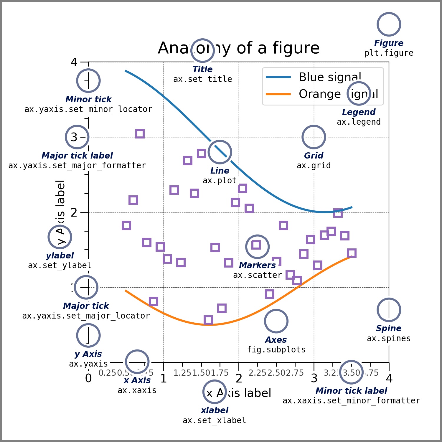
Visualization
Data visualization is one essential step in data analysis. There are many libraries that can be used to generate visualizations in python. The following is a short list to get you started.
- Matplotlib is the most widely used library
- Seaborn buids on top of matplotlib to generate more polished plots
- Plotly is known for its application in creating interactive visualizations
- Bokeh uses The Grammer of Graphics like ggplot but it’s native to python
We are going to use the same data set used in Wednesday’s R session for some examples of visualization in python.
[Input:]
# load python modules
import pandas as pd
import seaborn as sns
import matplotlib.pyplot as plt

# read in the birth weight data and the miRNA expression data using the url or from your local copy
bw = pd.read_csv("https://raw.githubusercontent.com/ucdavis-bioinformatics-training/2022_February_Introduction_to_R_for_Bioinformatics/main/birthweight.csv")
mir = pd.read_csv("https://raw.githubusercontent.com/ucdavis-bioinformatics-training/2022_February_Introduction_to_R_for_Bioinformatics/main/miRNA.csv")
[Input:]
display(bw.head(8))
[Output:]
     ID birth.date     location  length  birthweight  head.circumference  \
0  1107  1/25/1967      General      52         3.23                  36
1   697   2/6/1967  Silver Hill      48         3.03                  35
2  1683  2/14/1967  Silver Hill      53         3.35                  33
3    27   3/9/1967  Silver Hill      53         3.55                  37
4  1522  3/13/1967     Memorial      50         2.74                  33
5   569  3/23/1967     Memorial      50         2.51                  35
6   365  4/23/1967     Memorial      52         3.53                  37
7   808   5/5/1967  Silver Hill      48         2.92                  33

   weeks.gestation smoker  maternal.age  maternal.cigarettes  maternal.height  \
0               38     no            31                    0              164
1               39     no            27                    0              162
2               41     no            27                    0              164
3               41    yes            37                   25              161
4               39    yes            21                   17              156
5               39    yes            22                    7              159
6               40    yes            26                   25              170
7               34     no            26                    0              167

   maternal.prepregnant.weight  paternal.age  paternal.education  \
0                           57           NaN                 NaN
1                           62          27.0                14.0
2                           62          37.0                14.0
3                           66          46.0                 NaN
4                           53          24.0                12.0
5                           52          23.0                14.0
6                           62          30.0                10.0
7                           64          25.0                12.0

   paternal.cigarettes  paternal.height  low.birthweight  geriatric.pregnancy
0                  NaN              NaN                0                False
1                  0.0            178.0                0                False
2                  0.0            170.0                0                False
3                  0.0            175.0                0                 True
4                  7.0            179.0                0                False
5                 25.0              NaN                1                False
6                 25.0            181.0                0                False
7                 25.0            175.0                0                False
[Input:]
display(mir.head(8))
[Output:]
  Unnamed: 0  sample.27  sample.1522  sample.569  sample.365  sample.1369  \
0     miR-16         46           56          47          54           56
1     miR-21         52           43          40          35           59
2   miR-146a         98           97          87          96           84
3    miR-182         53           45          63          41           46

   sample.1023  sample.1272  sample.1262  sample.575  ...  sample.1360  \
0           59           49           55          62  ...           70
1           47           42           45          55  ...           57
2           96           88           97          96  ...          111
3           50           49           50          62  ...           46

   sample.1058  sample.755  sample.462  sample.1088  sample.553  sample.1191  \
0           77          56          65           42          63           66
1           55          46          58           54          54           48
2          124         101         101          107         106          102
3           56          50          60           63          60           50

   sample.1313  sample.1600  sample.1187
0           64           50           57
1           47           44           46
2          104          111           86
3           42           67           43

[4 rows x 43 columns]
It looks that the miRNA expression table uses the miRNA names as row names. We can tell the read_csv function to use the first column as the row names.
[Input:]
mir = pd.read_csv("https://raw.githubusercontent.com/ucdavis-bioinformatics-training/2022_February_Introduction_to_R_for_Bioinformatics/main/miRNA.csv", index_col = 0)
display(mir.head(8))
[Output:]
          sample.27  sample.1522  sample.569  sample.365  sample.1369  \
miR-16           46           56          47          54           56
miR-21           52           43          40          35           59
miR-146a         98           97          87          96           84
miR-182          53           45          63          41           46

          sample.1023  sample.1272  sample.1262  sample.575  sample.792  ...  \
miR-16             59           49           55          62          63  ...
miR-21             47           42           45          55          45  ...
miR-146a           96           88           97          96         104  ...
miR-182            50           49           50          62          51  ...

          sample.1360  sample.1058  sample.755  sample.462  sample.1088  \
miR-16             70           77          56          65           42
miR-21             57           55          46          58           54
miR-146a          111          124         101         101          107
miR-182            46           56          50          60           63

          sample.553  sample.1191  sample.1313  sample.1600  sample.1187
miR-16            63           66           64           50           57
miR-21            54           48           47           44           46
miR-146a         106          102          104          111           86
miR-182           60           50           42           67           43

[4 rows x 42 columns]
[Input:]
mir_trans = mir.T
display(mir_trans.head(8))
[Output:]
             miR-16  miR-21  miR-146a  miR-182
sample.27        46      52        98       53
sample.1522      56      43        97       45
sample.569       47      40        87       63
sample.365       54      35        96       41
sample.1369      56      59        84       46
sample.1023      59      47        96       50
sample.1272      49      42        88       49
sample.1262      55      45        97       50
In order to merge the two dataframes, we will insert a column into the transposed miRNA expression dataframe with the sample IDs. First, let’s check what data type does the ID column is in the birth weight dataframe.
[Input:]
bw.dtypes
[Output:]
ID                               int64
birth.date                      object
location                        object
length                           int64
birthweight                    float64
head.circumference               int64
weeks.gestation                  int64
smoker                          object
maternal.age                     int64
maternal.cigarettes              int64
maternal.height                  int64
maternal.prepregnant.weight      int64
paternal.age                   float64
paternal.education             float64
paternal.cigarettes            float64
paternal.height                float64
low.birthweight                  int64
geriatric.pregnancy               bool
dtype: object
[Input:]
mir_trans.insert(loc = 0, column = "ID", value = [int(INDEX.split(".")[1]) for INDEX in mir_trans.index])
display(mir_trans.head(8))
[Output:]
               ID  miR-16  miR-21  miR-146a  miR-182
sample.27      27      46      52        98       53
sample.1522  1522      56      43        97       45
sample.569    569      47      40        87       63
sample.365    365      54      35        96       41
sample.1369  1369      56      59        84       46
sample.1023  1023      59      47        96       50
sample.1272  1272      49      42        88       49
sample.1262  1262      55      45        97       50
[Input:]
mir_trans.dtypes
[Output:]
ID          int64
miR-16      int64
miR-21      int64
miR-146a    int64
miR-182     int64
dtype: object
[Input:]
# merge the two dataframes
data = pd.merge(bw, mir_trans, on = "ID", how = "inner")
display(data.head(8))
[Output:]
     ID birth.date     location  length  birthweight  head.circumference  \
0  1107  1/25/1967      General      52         3.23                  36
1   697   2/6/1967  Silver Hill      48         3.03                  35
2  1683  2/14/1967  Silver Hill      53         3.35                  33
3    27   3/9/1967  Silver Hill      53         3.55                  37
4  1522  3/13/1967     Memorial      50         2.74                  33
5   569  3/23/1967     Memorial      50         2.51                  35
6   365  4/23/1967     Memorial      52         3.53                  37
7   808   5/5/1967  Silver Hill      48         2.92                  33

   weeks.gestation smoker  maternal.age  maternal.cigarettes  ...  \
0               38     no            31                    0  ...
1               39     no            27                    0  ...
2               41     no            27                    0  ...
3               41    yes            37                   25  ...
4               39    yes            21                   17  ...
5               39    yes            22                    7  ...
6               40    yes            26                   25  ...
7               34     no            26                    0  ...

   paternal.age  paternal.education  paternal.cigarettes  paternal.height  \
0           NaN                 NaN                  NaN              NaN
1          27.0                14.0                  0.0            178.0
2          37.0                14.0                  0.0            170.0
3          46.0                 NaN                  0.0            175.0
4          24.0                12.0                  7.0            179.0
5          23.0                14.0                 25.0              NaN
6          30.0                10.0                 25.0            181.0
7          25.0                12.0                 25.0            175.0

   low.birthweight  geriatric.pregnancy  miR-16  miR-21  miR-146a  miR-182
0                0                False      57      49       116       48
1                0                False      68      47        98       57
2                0                False      49      48        98       55
3                0                 True      46      52        98       53
4                0                False      56      43        97       45
5                1                False      47      40        87       63
6                0                False      54      35        96       41
7                0                False      59      56       101       74

[8 rows x 22 columns]
[Input:]
# enter matplotlib mode
%matplotlib

# Let's do some simple plot
data.boxplot(rot = 90)
[Output:]
Using matplotlib backend: module://matplotlib_inline.backend_inline
<Axes: >

Let’s use Seaborn library to generate some visualizations
Let’s take a look at the data distribution
[Input:]
# data distribution plots can be generated using displot() function
sns.displot(data, x = "birthweight")
[Output:]
<seaborn.axisgrid.FacetGrid at 0x320f2d940>

[Input:]
# One may define a different bin size from the default
sns.displot(data, x = "birthweight", hue = "location", multiple = "stack")
[Output:]
<seaborn.axisgrid.FacetGrid at 0x321309a90>

Let’s take a look at how to plot the relationship between some variables.
[Input:]
sns.relplot(data, x = "birthweight", y = "head.circumference", hue = "smoker")
[Output:]
<seaborn.axisgrid.FacetGrid at 0x3213aa0d0>

Up until now, we have been using the default theme for the visualization from matplotlib. Let’s switch to Seaborn’s default theme to see if there is any difference.
[Input:]
sns.set_theme()
[Input:]
sns.displot(data, x = "birthweight", hue = "location", multiple = "stack")
[Output:]
<seaborn.axisgrid.FacetGrid at 0x321441310>

[Input:]
sns.relplot(data, x = "birthweight", y = "head.circumference", hue = "smoker")
[Output:]
<seaborn.axisgrid.FacetGrid at 0x321501e50>

Faceted visualization
[Input:]
tidy_data = pd.melt(data[["ID", "smoker", "miR-16", "miR-21", "miR-146a", "miR-182"]], id_vars = ["ID", "smoker"])
display(tidy_data.head(8))
[Output:]
     ID smoker variable  value
0  1107     no   miR-16     57
1   697     no   miR-16     68
2  1683     no   miR-16     49
3    27    yes   miR-16     46
4  1522    yes   miR-16     56
5   569    yes   miR-16     47
6   365    yes   miR-16     54
7   808     no   miR-16     59
[Input:]
sns.catplot(tidy_data, x = "smoker", y = "value", col = "variable", hue = "smoker", kind = "violin")
[Output:]
<seaborn.axisgrid.FacetGrid at 0x3230087d0>

[Input:]
g = sns.catplot(data=tidy_data, x='smoker', y='value', col='variable', hue='smoker',
                kind='violin', col_wrap=4, height=6, aspect=1.2)

# Remove individual x-axis labels from each subplot
for ax in g.axes.flat:
    ax.set_xlabel('')
    ax.tick_params(axis='x', labelsize=16)  # x-axis tick labels
    ax.tick_params(axis='y', labelsize=16)  # y-axis tick labels

    # Remove the default title
    title_text = ax.get_title()
    ax.set_title('')

    # Add title inside the plot area
    ax.text(0.5, 0.95, title_text,
            transform=ax.transAxes,  # Use axes coordinates (0-1)
            fontsize=16,
            fontweight='bold',
            verticalalignment='top',
            horizontalalignment='center',
            bbox=dict(boxstyle='round', facecolor='white', alpha=0.7))  # Optional background box


# Add a single shared x-axis label
g.fig.text(0.5, 0.01, 'Mother smoking Status', ha='center', fontsize=18, fontweight='bold')

# Adjust layout to make room for the shared label
plt.subplots_adjust(bottom=0.12)
[Output:]
