
scRNA shiny app
- Installation
- Notes about practical usage of the app
- Tutorial
- A few extra notes and link to AWS resources
Installation
-
Enter the following into your Rconsole in Rstudio after finishing the Mapping_Comparison.Rmd (it is also located at the bottom of the file itself).
if (!any(rownames(installed.packages()) == "shiny")){ install.packages("shiny") } library(shiny) if (!any(rownames(installed.packages()) == "markdown")){ if (!requireNamespace("BiocManager", quietly = TRUE)) install.packages("BiocManager") BiocManager::install("markdown") } library(markdown) if (!any(rownames(installed.packages()) == "tidyr")){ if (!requireNamespace("BiocManager", quietly = TRUE)) install.packages("BiocManager") BiocManager::install("tidyr") } library(tidyr) download.file("https://github.com/ucdavis-bioinformatics/scRNA_shiny/archive/master.zip", "scRNA_shiny.zip") #zipf <- file.choose(new=FALSE) zipf <- "scRNA_shiny.zip" outdir <- "scRNA_shiny" unzip(zipf, exdir=outdir) saveRDS(experiment.aggregate, file = "shiny.rds") -
You will now see a new directory appear in the workshop directory called
scRNA_shiny: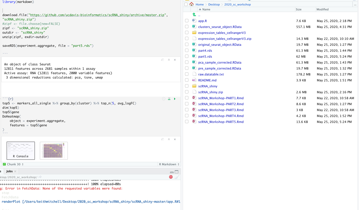
-
Navigate until you see the file
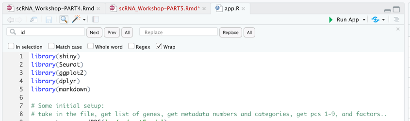
app.R. This is the file containing the app we will use for exploring the data. Open this file: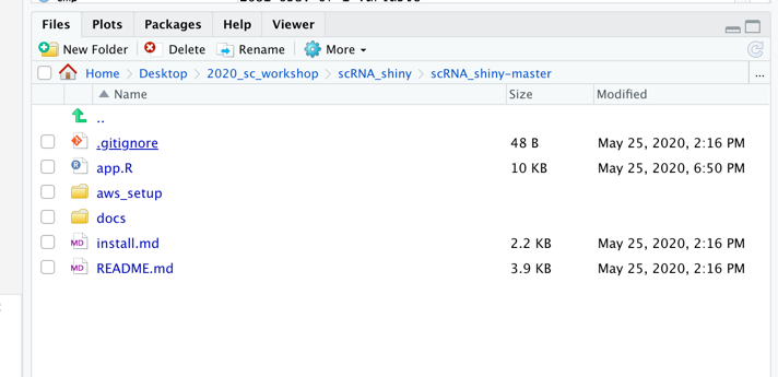
-
Now Click run app at the top of RStudio:
-
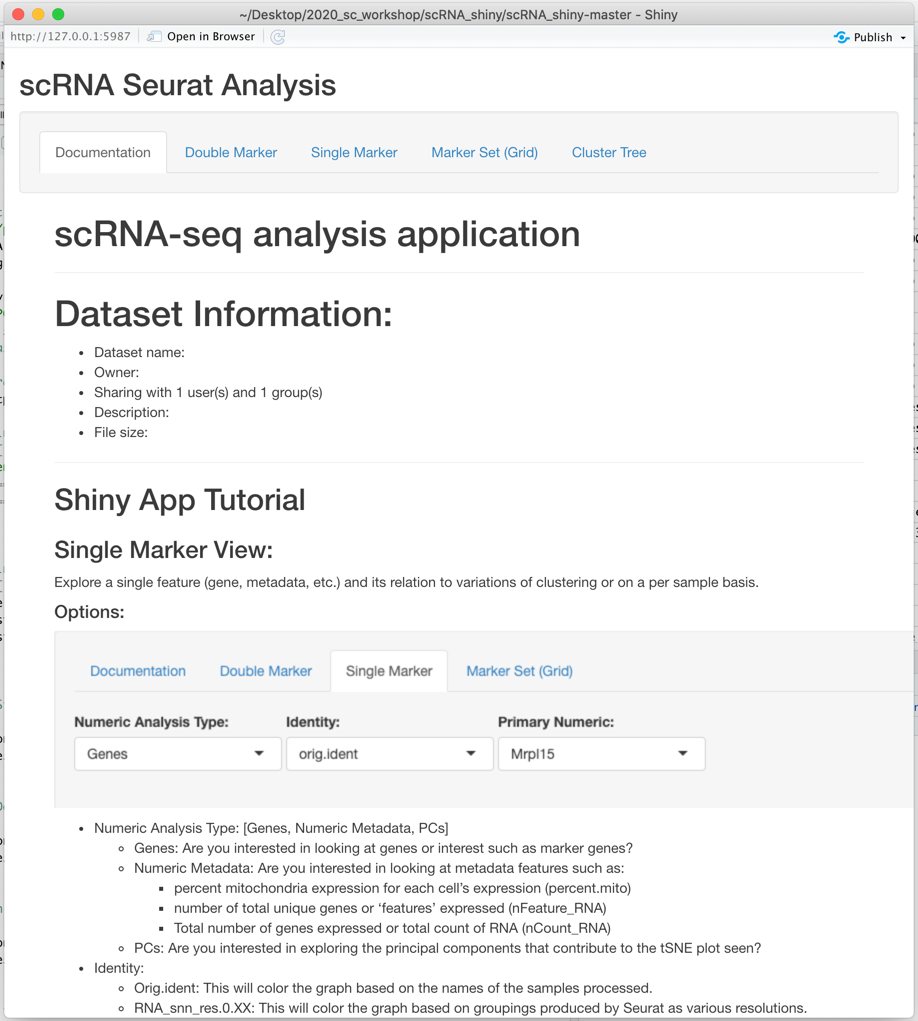
The app should now pop up in a new window:
App Practical Usage
This shiny app was created with the intention of working with biologists to extract meaning from the data by exploration. Usage of the app is not for creating finalized “publish ready” images but rather a means for enabling an analysis of potential clustering based on the marker genes of interest (the biological question). The app enables easier interaction with the data in order to explore what next steps can be taken towards producing “publish quality” images and which further analyses are relevant to the biological question.
Manual intervention (such as clustering) with the Seurat objects is often needed following this exploration. The hope is for the app to enables some of these capabilities in the near future. Lets do some exercises to see how might use the app to properly infer what custom clustering may need to be done.
Shiny App Tutorial
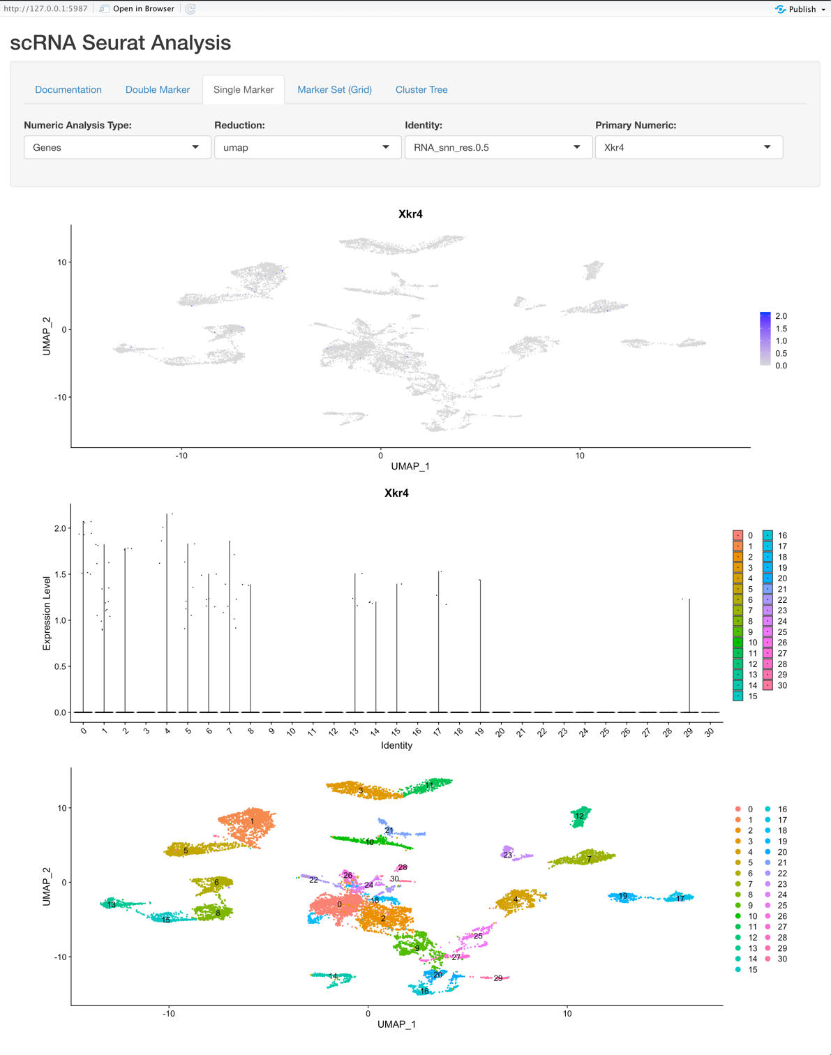
Single Marker View:
Explore a single feature (gene, metadata, etc.) and its relation to variations of clustering or on a per sample basis.
Options:
- Numeric Analysis Type: [Genes, Numeric Metadata, PCs]
- Genes: Are you interested in looking at genes or interest such as marker genes?
- Numeric Metadata: Are you interested in looking at metadata features such as:
- percent mitochondria expression for each cell’s expression (percent.mito)
- number of total unique genes or ‘features’ expressed (nFeature_RNA)
- Total number of genes expressed or total count of RNA (nCount_RNA)
- PCs: Are you interested in exploring the principal components that contribute to the tSNE plot seen?
- Reduction Type: [PCA, TSNE, UMAP]
- Identity:
- Orig.ident: This will color the graph based on the names of the samples processed.
- RNA_snn_res.0.XX: This will color the graph based on groupings produced by Seurat as various resolutions.
- A higher value of XX means that there is a higher resolution, and therefore more clusters or inferred groups of cell types.
- A lower value of XX means that there is a
- Primary Numeric: This will change to be Genes, Numeric Metadata, or PCs based on the value selected for ‘Numeric Analysis Type’.
Graphs:
- The first plot is a tSNE/PCA/UMAP that is colored based on the Primary Numeric selection.
- The second plot is a violin plot that displays the Identity selection on the X-axis and the Primary Numeric on the Y-axis.
- The third plot is the tSNE/PCA/UMAP that is colored based on the Identity selection.
Double Marker View:
Explore two features (gene, metadata, etc.) and its relation to variations of clustering or on a per sample basis.
Options: All of the options here are the same as the Single Marker View with the following field as an option.
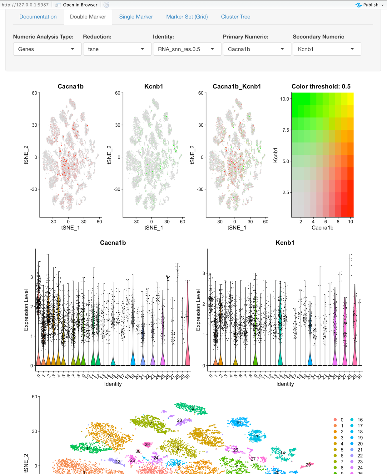
- Secondary Numeric: This, in combination with the Primary Numeric field enables a user to explore two Genes, Numeric Metadata, or PCs based on the value selected for ‘Numeric Analysis Type’.
Graphs:
- The first plot is a tSNE that is colored based on the Primary Numeric and Secondary Numeric selection.
- The second plot’s first tile is a violin plot that displays the Identity selection on the X-axis and the Primary Numeric on the Y-axis. The second plot’s second tile is the same as the first tile but is based on the selection of the Secondary Numeric field.
- The third plot is the tSNE that is colored based on the Identity selection.
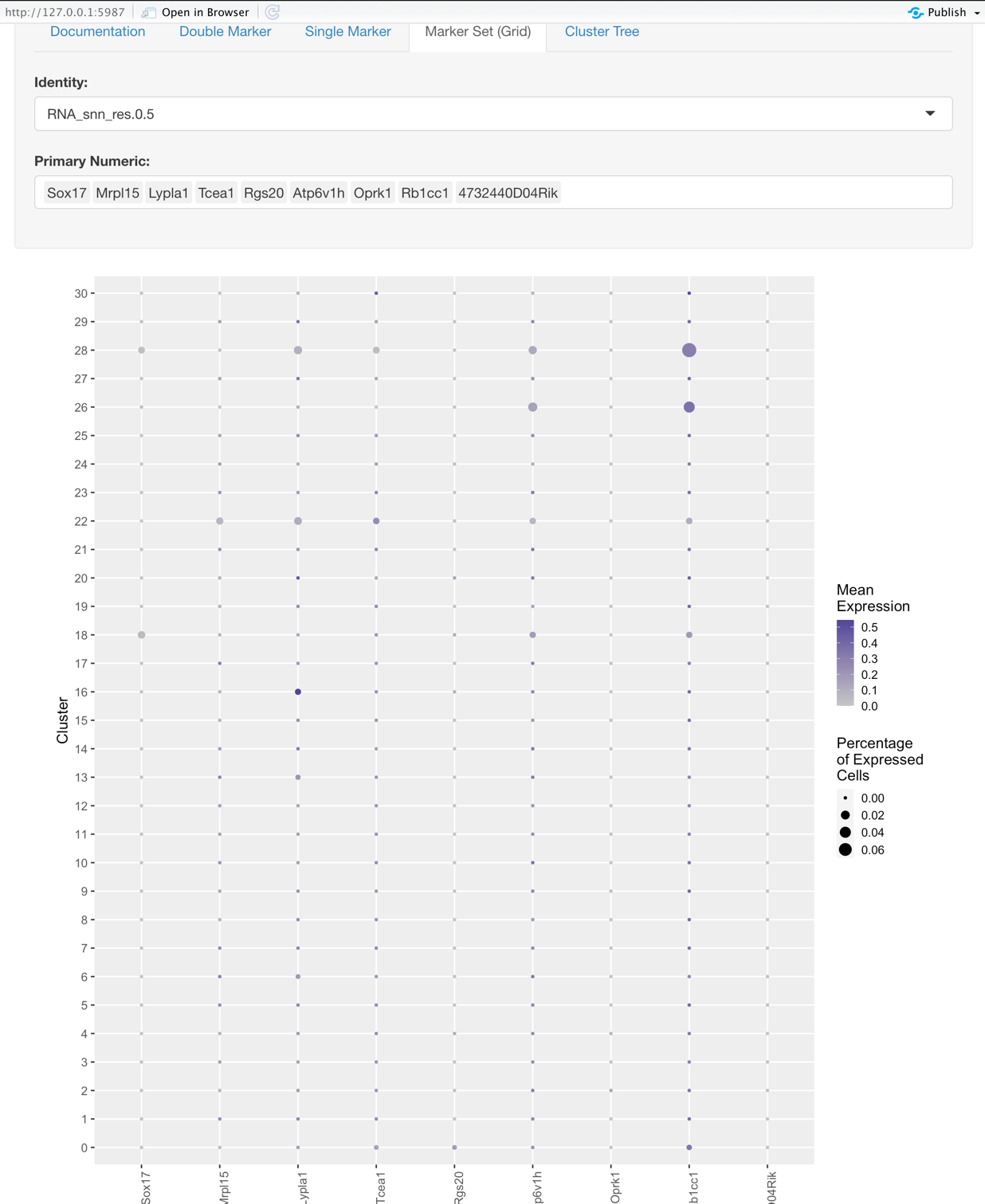
Marker Set (Grid)
This plot helps to explore sets of genes and their relation to the identity.
Options:
- Identity: the same as what is described for the Single Marker View
- Gene Selection: here you choose the set of genes you would like to explore based on the Identity selected.
Graph:
- Y-axis represents the Identity, such as the original samples or some groupings at a certain resolution.
- X-axis represents the genes selected. (Primary Numeric)
- The size of each dot on the grid represents the percentage of cells that expressed that gene.
- The color intensity of each dot on the grid represents the average expression of the cells that expressed a given gene.
- So what makes for a good marker gene for some given identity?
- High mean expression
- High percentage of cells expressing the gene
- Low mean expression and percentage of cells expressing the gene for the rest of the identities
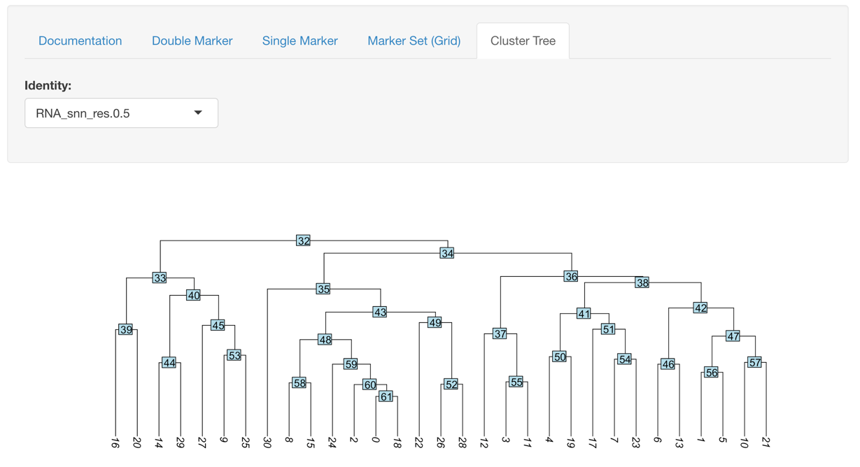
Cluster Tree Exploration
This plot helps to identify closest related clusters so when moving into the final analysis you have a better idea of what the real cell groups are in your samples.
Having trouble understanding what a tSNE vs UMAP plot represents?
- However, note that in our workflow we don’t cluster on the TSNE or UMAP coordinates, we cluster on the principal components and then use TSNE or UMAP for display, so the difference is purely visual.
- tSNE helpful video: https://www.youtube.com/watch?v=NEaUSP4YerM
- UMPA vs TSNE: https://towardsdatascience.com/tsne-vs-umap-global-structure-4d8045acba17
A few extra things:
- Your dataset is huge? You have to run analysis on an HPC and visualizing/interacting with your data is tricky via CLI.
AWS has huge instances you can run during the day for about 10$ with 100GB+ of RAM. You can just run it during working hours
when you can share the dataset with colleagues using a web hosted url, as it is billed hourly.
- If this is of interest to you feel free to reach out and check out the Shiny on AWS under Data Analysis in the docs.
-
You are working with someone where it may likely be difficult for them to download packages, Rstudio, the app etc. and you need to collaborate without being able to both access the same computer. AWS can help with this as well!
- With both of the above statements in mind, we will be trying to allow hosting of the app ont he Genome Center HPC in the near future so keep an eye out for that!