Metatranscriptomics data analysis

This document assumes preprocessing using HTStream has been completed.

The main objectives in metatranscriptomics data analysis is to answer the question: what are they doing. At the same time, it can also answer the question: who is there. These two concepts we have seen in the metagenomics data analysis part of this workshop. But we are going to see what is different when we have metatranscriptomics data.

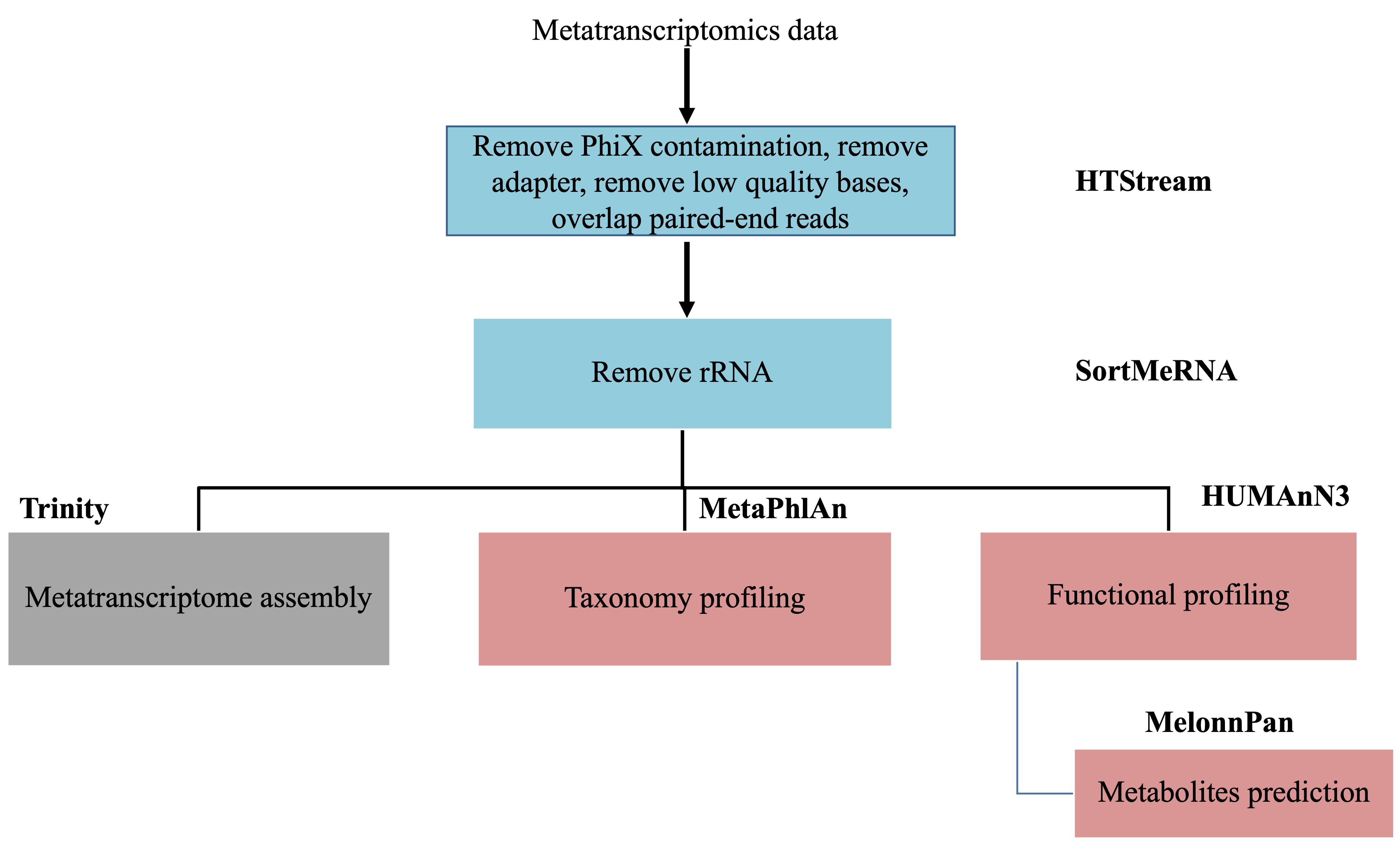
Remove/Separate rRNA

Ribosomal RNA is by far the most abundant form of RNA in most cells and can make up to 90% of the sequencing data. They perform essential cellular functions and offer information on a community’s structure and have been used in traditional taxonomic profiling of microbial communities. Nonetheless, they do not provide more information on a community. If one is mainly interested in studying the functional units of a microbial community, these rRNA provides little information and takes up the majority of computing resources if not removed.

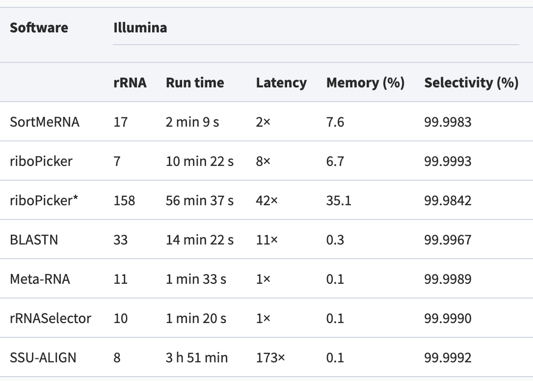
Li, etc., Microbiome 7,6 (2019), https://doi.org/10.1186/s40168-019-0618-5

There are many packages created to perform this task. They all attempt to match the sequencing reads to sequences in rRNA databases. They vary wildly in the requirement for computing resources, but have similar accuracy. We are going to use the more popular package that I have seen: SortMeRNA.

Performance comparison among methods:

SortMeRNA algorithm:

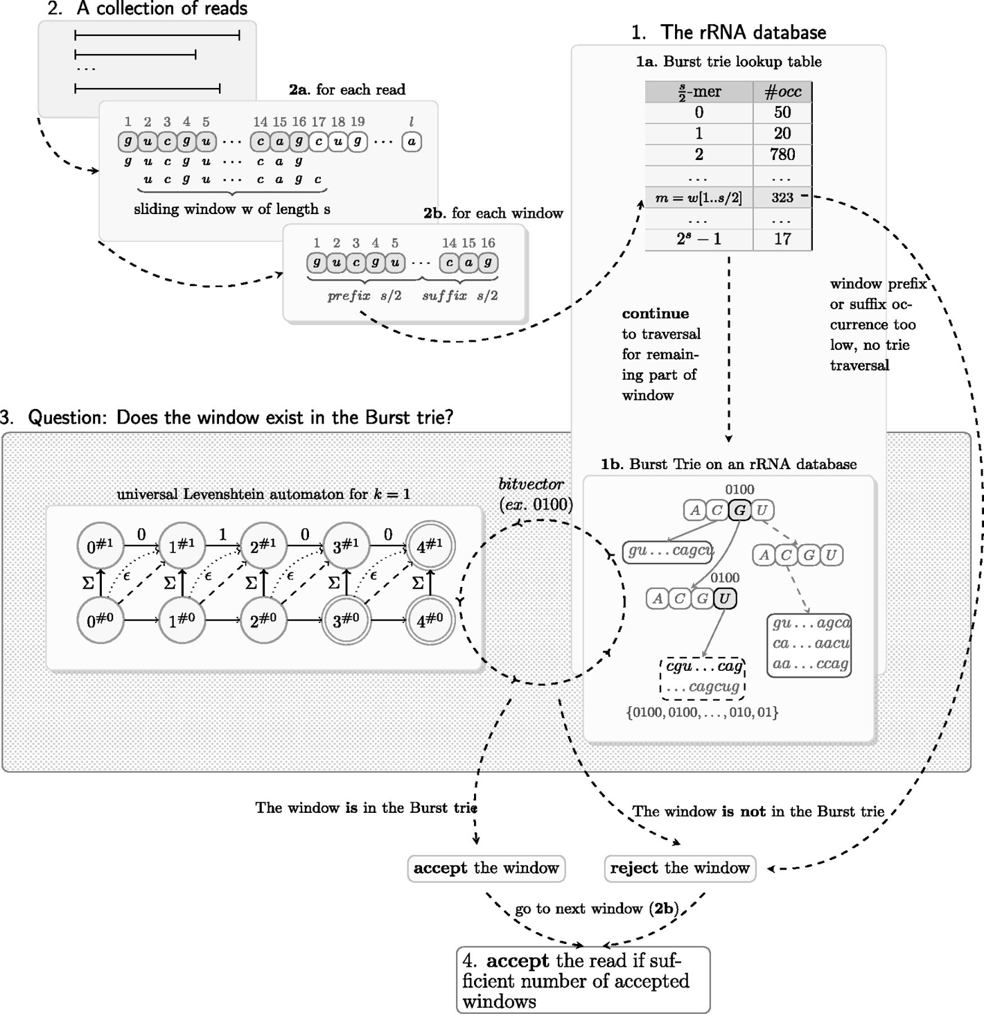
Li, etc., Microbiome 7,6 (2019), https://doi.org/10.1186/s40168-019-0618-5

In order to remove the rRNA fragements from our reads, we first need to have a database of all rRNA sequences that the software can use to compare our reads to. The one major rRNA database is SILVA, which holds quality checked and regularly updated rRNA sequence data. It includes both small (16S/18S)and large (23S/28S) subunit rRNA sequences for Bacteria, Archaea, and Eukarya. Rfam is another RNA resource that has some complementary rRNA sequences (5S, 5.8S). We are going to provide the combination of these rRNA sequences to SortMeRNA to remove any rRNA reads from our data.

Start Exercise 1:

First we are going to skip the step of downloading the rRNA database files, as they are large. Instead, we are going to link to the files that I have downloaded.

cd /share/workshop/meta_workshop/$USER/meta_example/References
ln -s /share/workshop/meta_workshop/jli/meta_example/References/SILVA* .
ln -s /share/workshop/meta_workshop/jli/meta_example/References/RF00* .
ls

Let’s load the module for SortMeRNA and take a look at the help manual.

module load sortmerna/4.3.4
sortmerna --help

Let’s go back to our scripts directory and download the slurm script to run SortMeRNA.

cd /share/workshop/meta_workshop/$USER/meta_example/scripts
wget https://ucdavis-bioinformatics-training.github.io/2021-December-Metagenomics-and-Metatranscriptomics/software_scripts/scripts/sortmerna.slurm
cat sortmerna.slurm

Now, we are ready to submit a few jobs. The jobs will take about 2 hours to run. But we can link available results over so that we can take a look at what results are generated by SortMeRNA. Pick one sample and see what outputs there are.

sbatch -J srna.${USER} --array=1-2 sortmerna.slurm mRNA

cd /share/workshop/meta_workshop/$USER/meta_example/
for i in {1..48}
do
  sample=$(sed "${i}q;d" scripts/samples.txt)
  mkdir -p 02-mRNA-rRNArmvd/${sample}
  ln -s /share/workshop/meta_workshop/jli/meta_example/02-mRNA-rRNArmvd/${sample}/${sample}.fq.gz 02-mRNA-rRNArmvd/${sample}/.
  ln -s /share/workshop/meta_workshop/jli/meta_example/02-mRNA-rRNArmvd/${sample}/out 02-mRNA-rRNArmvd/${sample}/.
done

Using the following commands, we can generate a summary file for the result of SortMeRNA.

cd /share/workshop/meta_workshop/$USER/meta_example/scripts

echo -e "Samples\tInput_reads\tPercent_rRNA\t\tPercent_LSU\tPercent_SSU\tPercent_5S\tPercent_5_8S\tOutput_reads"

for i in {1..48}
do
  sample=$(sed "${i}q;d" samples.txt)
  inrds=$(egrep "Total reads =" ../02-mRNA-rRNArmvd/${sample}/out/aligned.log |awk 'BEGIN{FS=" "}{print $NF}' - )
  covs=$(egrep -A4 "Coverage by database" ../02-mRNA-rRNArmvd/${sample}/out/aligned.log |tail -n +2 |awk 'BEGIN{FS=" ";ORS="\t"}{print $NF}' - )
  pcts=$(egrep "Total reads passing" ../02-mRNA-rRNArmvd/${sample}/out/aligned.log |awk 'BEGIN{FS="("}{print $2}' - |awk 'BEGIN{FS=")"}{print $1}' - )
  outrds=$(egrep "Total reads failing" ../02-mRNA-rRNArmvd/${sample}/out/aligned.log |awk 'BEGIN{FS="= "}{print $2}' - |awk 'BEGIN{FS=" "}{print $1}' - )
  echo -e "${sample}\t${inrds}\t${pcts}\t${covs}\t${outrds}"
done

End Exercise 1:

At this stage, we are ready to perform downstream analysis.

Assemble or Not?

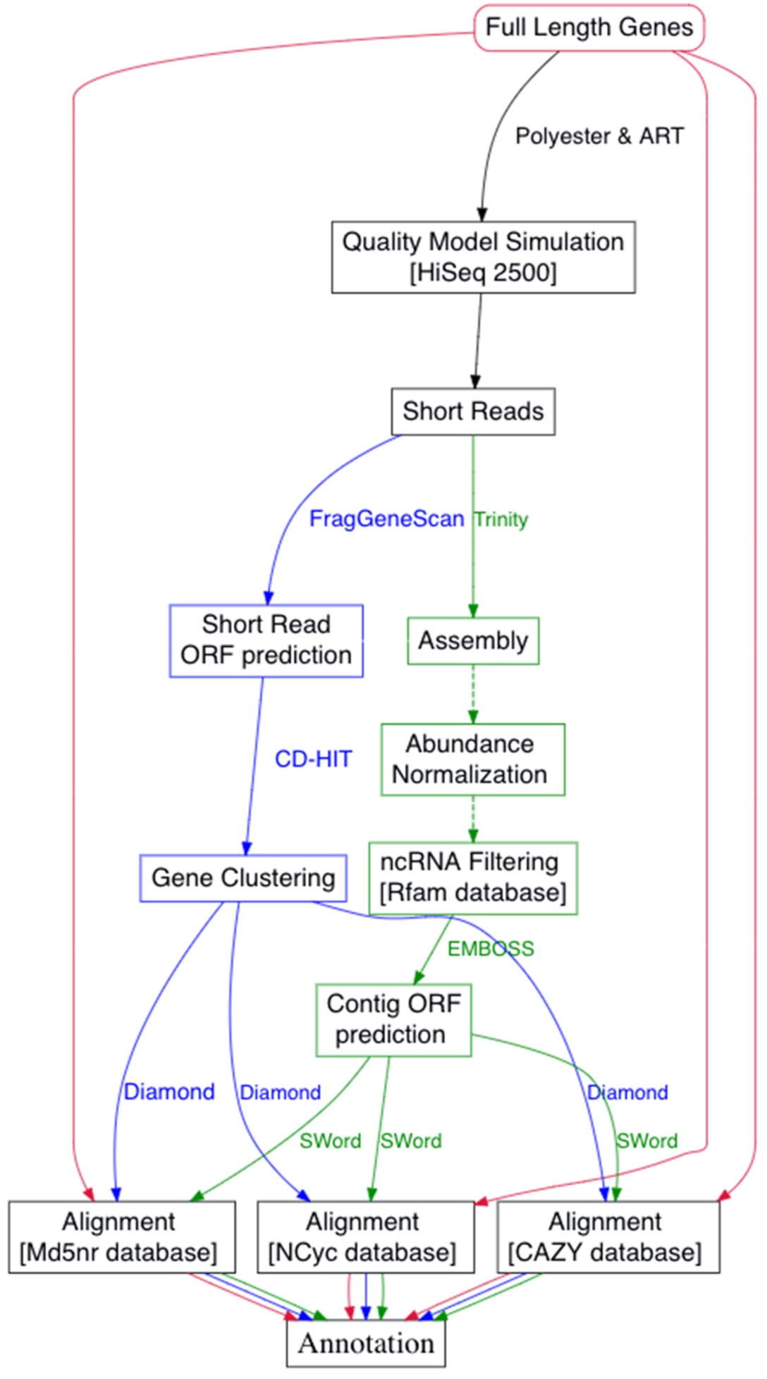
Anwar, etc., GigaScience, 8(8), 2019, https://doi.org/10.1093/gigascience/giz096

Introduction to Biobakery3

Biobakery3 is a suite of packages develped by a team of scientists from US and Italy (Harvard, US; Univ. of Trento, Italy; Broad Institute, US; Edmund Mach Foundation, Italy; IEO, Italy). It has integrated tools with improved methods for taxonomic, strain-level, functional, and phylogenetic profiling of metagenomes. All tools have extensive documentation on github. You can also find many tools developed for meta-omics data analysis on The Huttenhower Lab page.

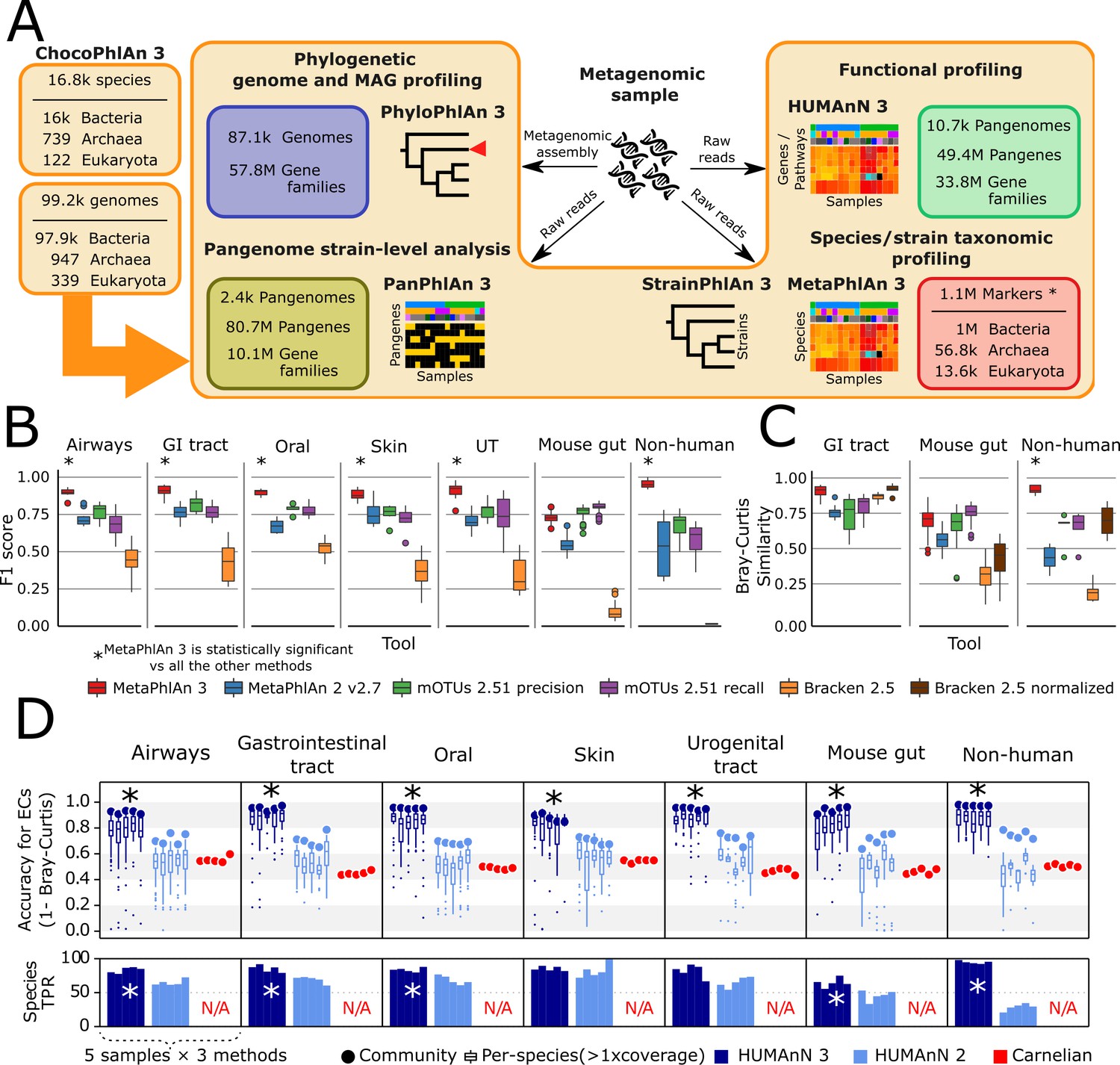
Beghini, etc., eLife 2021;10:e65088 DOI: 10.7554/eLife.65088

Taxonomic profiling

We have seen how to do taxonomic profiling using metagenomics data and k-mer based approach. Here we are going to take a look at MetaPhlAn3 (one of Biobakery’s tool set). It uses clade-specific marker genes, which are the set of genes that are shared among the strains in a clade, at the same time no other clades contains homologs close enough to incorrectly map reads. MetaPhlAn3 uses a set of 1.1M marker genes (including 61.8K viral markers) selected from a set of 16.8K species pangenomes.

Start Exercise 2:

Let’s take a look at the help manual of MetaPhlAn3.

This package runs quite fast, taking ~4-5 minutes for each job using 24 CPUs. Let’s submit some jobs.

cd /share/workshop/meta_workshop/$USER/meta_example/scripts
wget https://ucdavis-bioinformatics-training.github.io/2021-December-Metagenomics-and-Metatranscriptomics/software_scripts/scripts/metaphlan.slurm
cat metaphlan.slurm
sbatch -J mtp.${USER} --array=1-8 metaphlan.slurm
squeue -u ${USER}

Please take a look at the output directory of MetaPhlAn and the output files. What type of quantification MetaPhlAn produces?

We are going to use two packages to generate some visualization using the output from MetaPhlAn. First we are going to merge the output files from individual samples into one file. There is a python script in MetaPhlAn package to do that. So, we are going to load the module MetaPhlAn3 first. Always remember to read the message printed out after loading the module, as it may contain additional instructions to complete the process (such as required source activate for python packages).

module load metaphlan/3.0.13
source activate metaphlan-3.0.13

We are going to copy the MetaPhlAn results I generated on the full dataset. These are small files. Then we are going to run the merge script.

cd /share/workshop/meta_workshop/$USER/meta_example
cp -r /share/workshop/meta_workshop/jli/meta_example/original-03-Metaphlan-RNA ./03-Metaphlan-RNA
cd /share/workshop/meta_workshop/$USER/meta_example/03-Metaphlan-RNA
python /share/biocore/projects/Internal_Jessie_UCD/software/miniconda-metaphlan/miniconda3/lib/python3.7/site-packages/metaphlan/utils/merge_metaphlan_tables.py */*_profile.txt > merged_abundance_profile.txt

We can filter MetaPhlAn output for species specific abundance using the following commands.

cd /share/workshop/meta_workshop/$USER/meta_example/03-Metaphlan-RNA
grep -E "s__|clade" merged_abundance_profile.txt |sed 's/^.*s__//g' |cut -f1,3- |sed -e 's/clade_name/samples/g' |sed -e 's/_profile//g' > merged_abundance_species.txt

Once we have this combined abundance file, we can create some visualization to inspect and see whether it matches with our expectations. First, we are going to filter the file to create an abundance table for species level, then we will generate a heatmap. (Because of the small dataset, the

module load hclust2/1.0.0
source activate hclust2-1.0.0
cd /share/workshop/meta_workshop/$USER/meta_example/03-Metaphlan-RNA
hclust2.py -i merged_abundance_species.txt --f_dist_f braycurtis --s_dist_f braycurtis -o heatmap_species.png

The above commands has produced a heatmap.

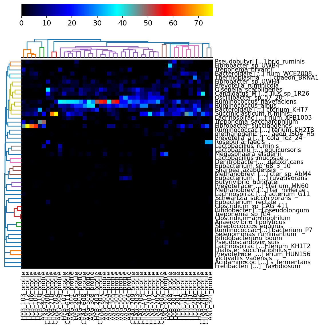
The following commands will generate a cladogram using the abundance table.

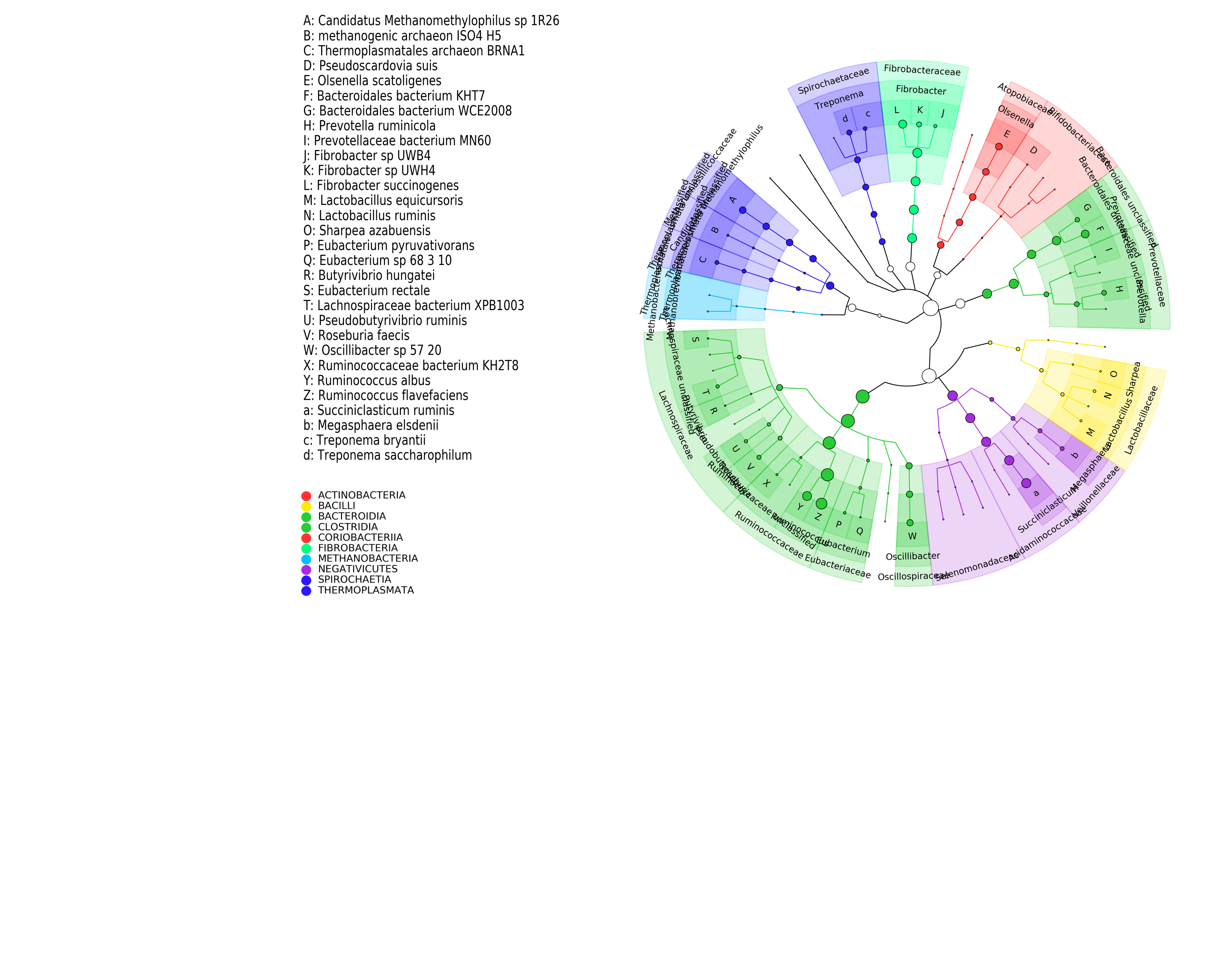
module load graphlan/1.1.3
source activate graphlan-1.1.3
cd /share/workshop/meta_workshop/$USER/meta_example/03-Metaphlan-RNA

tail -n +2 merged_abundance_profile.txt |cut -f1,3- > merged_abundance_reformated.txt

export2graphlan.py --skip_rows 1 -i merged_abundance_reformated.txt --tree merged_abundance.tree.txt --annotation merged_abundance.anno.txt --most_abundant 100 --abundance_threshold 1 --least_biomarkers 10 --annotations 5,6 --external_annotations 7 --min_clade_size 1

graphlan_annotate.py --annot merged_abundance.anno.txt merged_abundance.tree.txt merged_abundance.xml

graphlan.py --dpi 300 merged_abundance.xml merged_abundance.png --external_legends

End Exercise 2:

We are going to use MaAsLin2 to perform some differential abundance analysis. This time, we are using the relative abundance produced by MetaPhlAn3. We will download the merged abundance table at species level to our laptop. Open RStudio and install MaAsLin2 if you haven’t done so.

Start Exercise 3:

if (!requireNamespace("BiocManager", quietly = TRUE))
  install.packages("BiocManager")

if (!any(rownames(installed.packages()) == "Maaslin2")){
  BiocManager::install("Maaslin2")
}
library(Maaslin2)

abundance <- read.table(file="./merged_abundance_species.txt", sep="\t", header=T, stringsAsFactors=F)
rownames(abundance) <- abundance$samples
abundance <- abundance[,-1]
colnames(abundance) <- gsub("_profile", "", colnames(abundance))

pdata <- read.table(file="./feed.txt", sep="\t", header=F, stringsAsFactors=F)
colnames(pdata) <- c("Samples", "Feed.Efficiency")
pdata$Breed <- sapply(pdata$Samples, function(x){strsplit(x, "_", fixed=T)[[1]][1]})
pdata$Breed <- factor(pdata$Breed, levels=c("ANG", "CHAR", "HYB"))
pdata$Feed.Efficiency <- factor(pdata$Feed.Efficiency, levels=c("L", "H"))

pdata$samp2 <- pdata$Samples

# Reorder pdata to match colnames of abundance
pdata <- left_join(data.frame(samp2 = colnames(abundance)), pdata)
identical(pdata$samp2, colnames(abundance))
rownames(pdata) <- pdata$Samples

Maaslin2(input_data=abundance, input_metadata=pdata, output="maaslin", fixed_effects=c("Breed", "Feed.Efficiency"), reference=c("Breed, ANG", "Feed.Efficiency, L"), min_prevalence=0.001)

End Exercise 3:

Functional profiling I

Start Exercise 4:

We are going to perform functional profiling a second time using HUMAnN. This time you will write your own slurm script, using the one we have used for metagenomics data as a template. Please submit maximum 2 jobs once your script is ready. The goal is to obtain relative abundance table for those samples.

End Exercise 4:

Functional profiling II

Using another package from the Biobakery project, we are going to prodict metabolites using the result from the previous step (HUMAnN3). This MelonnPan package uses machine learning technique to achieve good prediction results. The module available in the package was trained on human gut microbial data, but the package offers the option to train your own model if you have data available for your specific microbial community. We are going to simply use the model from the package and do some predictions.

First, download the merged relative abundance table I have generated for all samples. Then we are going to install the package in RStudio.

The instructions are provided here. Just one way to do things. But please look through the github page and try to follow those instructions first.

Tada