
Last Updated: June 19, 2023
Part 1: Loading data from CellRanger into R
Our first Markdown document concentrates on getting data into R and setting up our initial object.
Single Cell Analysis with Seurat and some custom code!
Seurat (now Version 4) is a popular R package that is designed for QC, analysis, and exploration of single cell data. Seurat aims to enable users to identify and interpret sources of heterogeneity from single cell transcriptomic measurements, and to integrate diverse types of single cell data. Further, the authors provide several tutorials, on their website.
The expression_data_cellranger.zip file that we have downloaded in previous step contains the single cell matrix files and HDF5 files for three single nuclei RNASeq samples from Becker et al., 2022. After un-compressing the file, please make sure that you see three folders: A001-C-007, A001-C-104 and B001-A-301 in the same folder as this R markdown file.
We start each markdown document with loading needed libraries for R:
# must have Seurat
library(Seurat)
library(kableExtra)
library(ggplot2)
Setup the experiment folder and data info
experiment.name <- "Becker 2022 colorectal cancer continuum"
dataset.loc <- "./"
sample.ids <- c("A001-C-007", "A001-C-104", "B001-A-301")
Read in the cellranger sample metrics csv files
There is a single metrics summary file for each sample. The code in the box below reads in each of these files and creates a single table containing data from all of the samples.
sample.metrics <- lapply(sample.ids, function(id){
  metrics = read.csv(file.path(dataset.loc, paste0(id,"/outs"),"metrics_summary.csv"),
                     colClasses = "character")
})
experiment.metrics <- do.call("rbind", sample.metrics)
rownames(experiment.metrics) <- sample.ids

sequencing.metrics <- data.frame(t(experiment.metrics[,c(1:19)]))

rownames(sequencing.metrics) <- gsub("\\."," ", rownames(sequencing.metrics))

sequencing.metrics %>%
  kable(caption = 'Cell Ranger Results') %>%
  pack_rows("Overview", 1, 3, label_row_css = "background-color: #666; color: #fff;") %>%
  pack_rows("Sequencing Characteristics", 4, 9, label_row_css = "background-color: #666; color: #fff;") %>%
  pack_rows("Mapping Characteristics", 10, 19, label_row_css = "background-color: #666; color: #fff;") %>%
  kable_styling("striped")
| A001.C.007 | A001.C.104 | B001.A.301 | |
|---|---|---|---|
| Overview | |||
| Estimated Number of Cells | 1,796 | 3,142 | 4,514 |
| Mean Reads per Cell | 77,524 | 151,317 | 38,935 |
| Median Genes per Cell | 927 | 959 | 1,331 |
| Sequencing Characteristics | |||
| Number of Reads | 139,233,487 | 475,437,350 | 175,752,014 |
| Valid Barcodes | 97.4% | 95.4% | 98.5% |
| Sequencing Saturation | 75.5% | 84.3% | 69.0% |
| Q30 Bases in Barcode | 97.4% | 96.4% | 96.6% |
| Q30 Bases in RNA Read | 95.6% | 94.4% | 94.1% |
| Q30 Bases in UMI | 97.5% | 96.4% | 96.5% |
| Mapping Characteristics | |||
| Reads Mapped to Genome | 94.3% | 92.1% | 89.0% |
| Reads Mapped Confidently to Genome | 72.3% | 49.1% | 83.8% |
| Reads Mapped Confidently to Intergenic Regions | 8.2% | 7.4% | 5.0% |
| Reads Mapped Confidently to Intronic Regions | 26.9% | 20.6% | 40.2% |
| Reads Mapped Confidently to Exonic Regions | 37.2% | 21.2% | 38.6% |
| Reads Mapped Confidently to Transcriptome | 61.1% | 39.4% | 73.4% |
| Reads Mapped Antisense to Gene | 2.4% | 1.9% | 4.8% |
| Fraction Reads in Cells | 29.6% | 37.6% | 36.8% |
| Total Genes Detected | 23,930 | 25,326 | 25,462 |
| Median UMI Counts per Cell | 1,204 | 1,231 | 1,913 |
rm(sample.metrics, experiment.metrics, sequencing.metrics)
Load the Cell Ranger expression data and create the base Seurat object
Cell Ranger provides a function cellranger aggr that will combine multiple samples into a single matrix file. However, when processing data in R this is unnecessary and we can quickly aggregate them in R.
Load the expression matrix
First we read in data from each individual sample folder, using either the h5 file (first code block), or the matrix directory (second code block).
expression.data <- lapply(sample.ids, function(id){
  sample.matrix = Read10X_h5(file.path(dataset.loc, id, "/outs","filtered_feature_bc_matrix.h5"))
  colnames(sample.matrix) = paste(sapply(strsplit(colnames(sample.matrix),split="-"), '[[', 1L), id, sep="_")
  sample.matrix
})
names(expression.data) <- sample.ids

str(expression.data)
If you don’t have the needed hdf5 libraries, you can read in the matrix files using the Read10X function rather than the Read10X_h5 function. The resulting object is the same.
expression.data <- sapply(sample.ids, function(id){
  sample.matrix <- Read10X(file.path(dataset.loc, id, "/outs","filtered_feature_bc_matrix"))
  colnames(sample.matrix) <- paste(sapply(strsplit(colnames(sample.matrix), split="-"), '[[', 1L), id, sep="_")
  sample.matrix
})
names(expression.data) <- sample.ids

str(expression.data)
Create the Seurat object
The CreateSeuratObject function allows feature (gene) and cell filtering by minimum cell and feature counts. We will set these to 0 for now in order to explore manual filtering more fully in part 2.
aggregate.data <- do.call("cbind", expression.data)

experiment.aggregate <- CreateSeuratObject(
  aggregate.data,
  project = experiment.name,
  min.cells = 0,
  min.features = 0,
  names.field = 2, # tells Seurat which part of the cell identifier contains the sample name
  names.delim = "\\_")

experiment.aggregate
str(experiment.aggregate)
rm(expression.data, aggregate.data)
Understanding the Seurat object
A Seurat object is a complex data structure containing the data from a single cell or single nucleus assay and all of the information associated with the experiment, including annotations, analysis, and more. This data structure was developed by the authors of the Seurat analysis package, for use with their pipeline.
Most Seurat functions take the object as an argument, and return either a new Seurat object or a ggplot object (a visualization). As the analysis continues, more and more data will be added to the object.
Let’s take a moment to explore the Seurat object.
slotNames(experiment.aggregate)
# a slot is accessed with the @ symbol
experiment.aggregate@assays
- Which slots are empty, and which contain data?
- What type of object is the content of the meta.data slot?
- What metadata is available?
There is often more than one way to interact with the information stored in each of a Seurat objects many slots. The default behaviors of different access functions are described in the help documentation.
# which slot is being accessed here? can you write another way to produce the same result?
head(experiment.aggregate[[]])
Explore the dataset
We will begin filtering and QA/QC in the next section. For now, let’s take a moment to explore the basic characteristics of our dataset.
Metadata by sample
Using base R functions we can take a quick look at the available metadata by sample.
table(experiment.aggregate$orig.ident)
tapply(experiment.aggregate$nCount_RNA, experiment.aggregate$orig.ident, summary)
tapply(experiment.aggregate$nFeature_RNA, experiment.aggregate$orig.ident, summary)
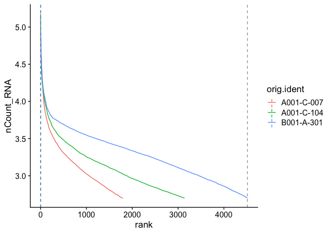
Barcode inflection plots
Imagine the barcode rank plot from the Cell Ranger web summary. That graphic plots the number of UMIs agains the barcode rank, and typically has a sharp inflection point where the number of UMIs drops dramatically. These points can represent a transition between cell types from a higher RNA content population to a lower RNA content population, or from cell-associated barcodes to background.
The Seurat BarcodeInflectionsPlot provides a similar graphic. In this case, because we are using the filtered barcode matrix, rather than all barcodes, much of the background is absent from the plot.
experiment.aggregate <- CalculateBarcodeInflections(experiment.aggregate)
BarcodeInflectionsPlot(experiment.aggregate)
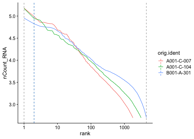
Adding a log-scale transformation to the x-axis increases the resemblance to the Cell Ranger plot. Values on the y-axis are already log-transformed.
BarcodeInflectionsPlot(experiment.aggregate) +
  scale_x_continuous(trans = "log10")
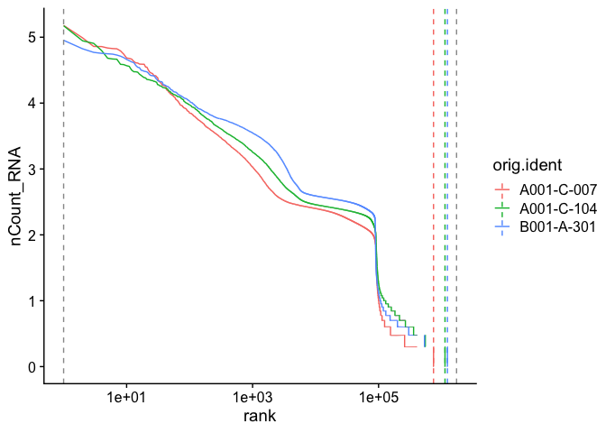
A barcode inflection plot calculated on all barcodes (the raw_feature_bc_matrix files) looks more like the familiar Cell Ranger barcode rank plot.
Reads from the mitochondrial genome
Filtering on the expression of genes from the mitochondrial genome is not appropriate in all cell types, however, in many tissues, low-quality / dying cells may exhibit extensive mitochondrial contamination. Even when not filtering on mitochondrial expression, the data can be interesting or informative.
The PercentageFeatureSet function calculates the proportion of counts originating from a set of features. Genes in the human mitochondrial genome begin with ‘MT’, while those in the mouse mitochondrial genome begin with ‘mt’. These naming conventions make calculating percent mitochondrial very straightforward.
experiment.aggregate$percent_MT <- PercentageFeatureSet(experiment.aggregate, pattern = "^MT-")
summary(experiment.aggregate$percent_MT)
Save the object and download the next Rmd file
saveRDS(experiment.aggregate, file="scRNA_workshop_1.rds")
download.file("https://raw.githubusercontent.com/ucdavis-bioinformatics-training/2023-June-Single-Cell-RNA-Seq-Analysis/main/data_analysis/scRNA_Workshop-PART2.Rmd", "scRNA_Workshop-PART2.Rmd")
Session Information
sessionInfo()