
Last Updated: June 20, 2023
Part 4: Clustering
Setup
Load the required libraries and read in the saved object from the previous section.
library(Seurat)
library(kableExtra)
library(tidyr)
library(dplyr)
library(ggplot2)
library(dplyr)

experiment.aggregate <- readRDS("scRNA_workshop_3.rds")
experiment.aggregate
set.seed(12345)
Select compenents
In the previous section, we looked at the principal components analysis in a number of different ways. Now we need to select the components that will be used in the following steps (dimensionality reduction by UMAP or tSNE and clustering). If we use too few components, we risk leaving out interesting variation that may define cell types. What happens if we use too many? A greater number of PCs will increase the computational time of following steps.
Lets choose the first 50, based on the elbow plot from the last section.
use.pcs <- 1:50
Cluster
Seurat implements an graph-based clustering approach. Distances between the cells are calculated based on previously identified PCs.
The default method for identifying k-nearest neighbors has been changed in V4 to annoy (“Approximate Nearest Neighbors Oh Yeah!). This is an approximate nearest-neighbor approach that is widely used for high-dimensional analysis in many fields, including single-cell analysis. Extensive community benchmarking has shown that annoy substantially improves the speed and memory requirements of neighbor discovery, with negligible impact to downstream results.
Seurat prior approach was heavily inspired by recent manuscripts which applied graph-based clustering approaches to scRNAseq data. Briefly, Seurat identified clusters of cells by a shared nearest neighbor (SNN) modularity optimization based clustering algorithm. First calculate k-nearest neighbors (KNN) and construct the SNN graph. Then optimize the modularity function to determine clusters. For a full description of the algorithms, see Waltman and van Eck (2013) The European Physical Journal B. You can switch back to using the previous default setting using nn.method=”rann”.
The FindClusters function implements the neighbor based clustering procedure, and contains a resolution parameter that sets the granularity of the downstream clustering, with increased values leading to a greater number of clusters. This code produces a series of resolutions for us to investigate and choose from.
?FindNeighbors
experiment.aggregate <- FindNeighbors(experiment.aggregate, reduction = "pca", dims = use.pcs)
experiment.aggregate <- FindClusters(experiment.aggregate,
                                     resolution = seq(0.25, 4, 0.5))
Seurat adds the clustering information to the metadata beginning with “RNA_snn_res.” followed by the resolution.
head(experiment.aggregate@meta.data) %>%
  kable(caption = 'Cluster identities are added to the meta.data slot.') %>%
  kable_styling("striped")
| orig.ident | nCount_RNA | nFeature_RNA | percent_MT | S.Score | G2M.Score | Phase | old.ident | RNA_snn_res.0.25 | RNA_snn_res.0.75 | RNA_snn_res.1.25 | RNA_snn_res.1.75 | RNA_snn_res.2.25 | RNA_snn_res.2.75 | RNA_snn_res.3.25 | RNA_snn_res.3.75 | seurat_clusters | |
|---|---|---|---|---|---|---|---|---|---|---|---|---|---|---|---|---|---|
| AAACCCAAGTTATGGA_A001-C-007 | A001-C-007 | 2024 | 1496 | 0.5774783 | 0.0287929 | -0.1413033 | S | A001-C-007 | 5 | 8 | 10 | 10 | 10 | 21 | 20 | 21 | 21 |
| AAACGCTTCTCTGCTG_A001-C-007 | A001-C-007 | 1401 | 1036 | 1.1486486 | 0.2739756 | 0.8777017 | G2M | A001-C-007 | 9 | 14 | 18 | 20 | 22 | 24 | 24 | 25 | 25 |
| AAAGAACGTGCTTATG_A001-C-007 | A001-C-007 | 1624 | 1125 | 0.4219409 | -0.0702453 | -0.0551464 | G1 | A001-C-007 | 5 | 8 | 10 | 10 | 10 | 20 | 19 | 19 | 19 |
| AAAGAACGTTTCGCTC_A001-C-007 | A001-C-007 | 1683 | 1177 | 0.4595060 | 0.0843744 | 1.0192889 | G2M | A001-C-007 | 4 | 2 | 14 | 16 | 18 | 18 | 18 | 18 | 18 |
| AAAGGATTCATTACCT_A001-C-007 | A001-C-007 | 1178 | 936 | 0.8176615 | -0.0128403 | 0.1327610 | G2M | A001-C-007 | 4 | 2 | 14 | 16 | 18 | 18 | 18 | 18 | 18 |
| AAAGTGACACGCTTAA_A001-C-007 | A001-C-007 | 2701 | 1779 | 0.3259689 | -0.0803025 | 0.0327879 | G2M | A001-C-007 | 5 | 8 | 10 | 10 | 10 | 21 | 20 | 21 | 21 |
Explore clustering resolutions
Lets first investigate how many clusters each resolution produces and set it to the smallest resolutions of 0.5 (fewest clusters).
cluster.resolutions <- grep("res", colnames(experiment.aggregate@meta.data), value = TRUE)
sapply(cluster.resolutions, function(x) length(levels(experiment.aggregate@meta.data[,x])))
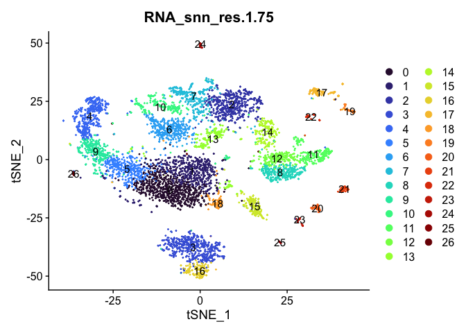
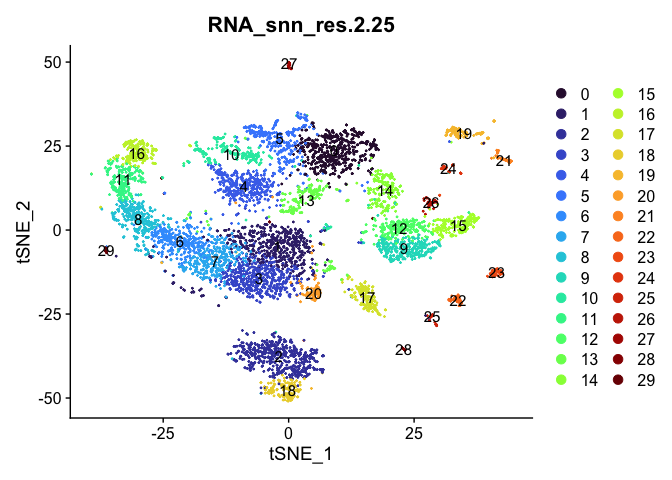
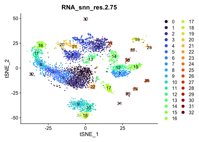
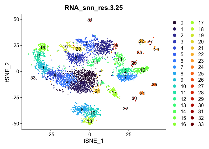
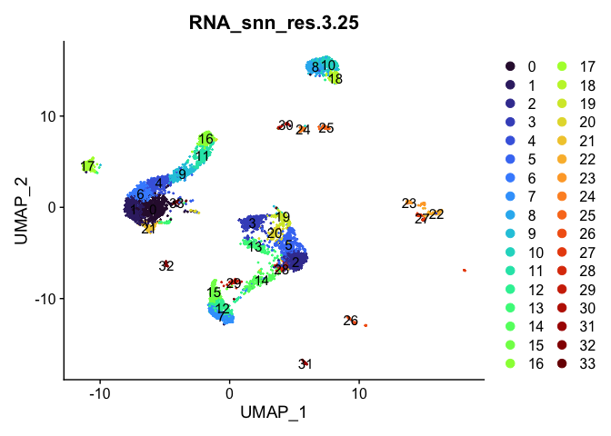
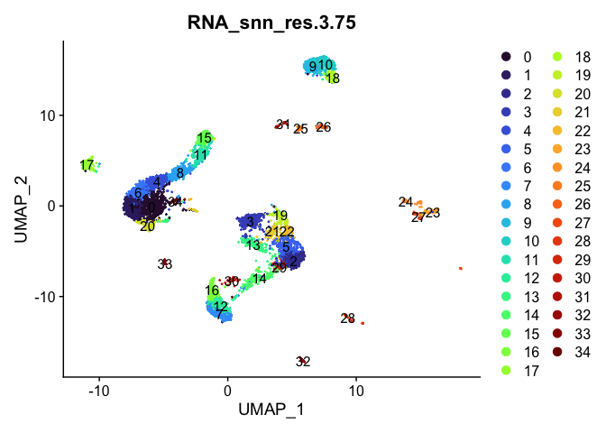
Visualize clustering
Dimensionality reduction plots can be used to visualize the clustering results. On these plots, we can see how each clustering resolution aligns with patterns in the data revealed by dimensionality reductions.
tSNE
# calculate tSNE
experiment.aggregate <- RunTSNE(experiment.aggregate,
reduction.use = "pca",
dims = use.pcs,
do.fast = TRUE)
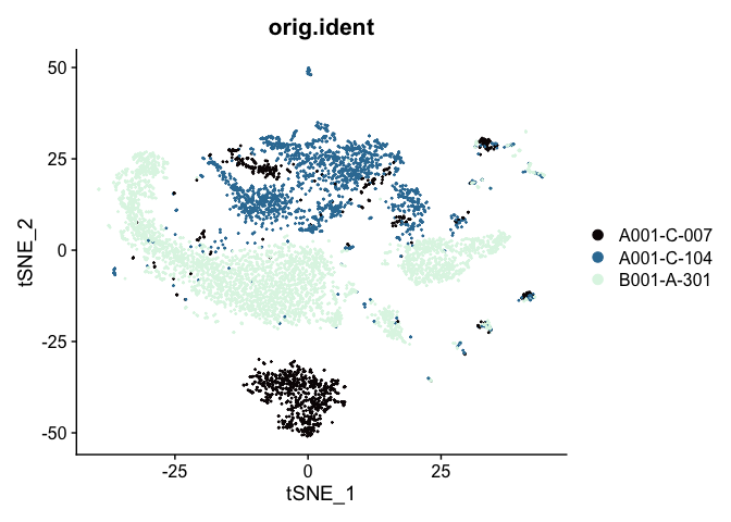
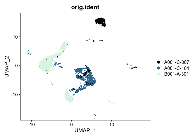
# tSNE colored by sample identity
DimPlot(experiment.aggregate,
group.by = "orig.ident",
reduction = "tsne",
shuffle = TRUE) +
scale_color_viridis_d(option = "mako")
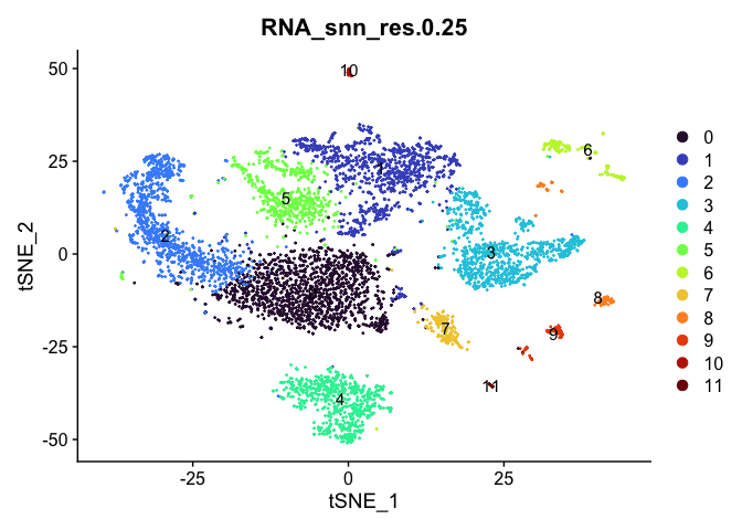
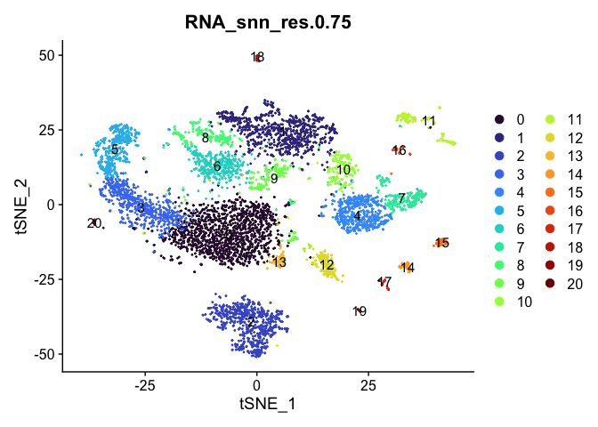
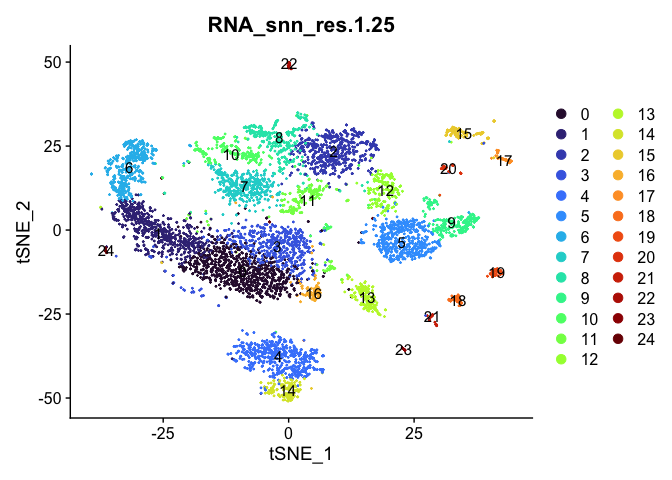
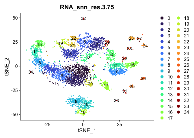
# tSNE colored by cluster
lapply(cluster.resolutions, function(res){
  DimPlot(experiment.aggregate,
          group.by = res,
          reduction = "tsne",
          label = TRUE,
          shuffle = TRUE) +
    scale_color_viridis_d(option = "turbo")
})
UMAP
# calculate UMAP
experiment.aggregate <- RunUMAP(experiment.aggregate,
                                dims = use.pcs)
# UMAP colored by sample identity
DimPlot(experiment.aggregate,
        group.by = "orig.ident",
        reduction = "umap",
        shuffle = TRUE) +
  scale_color_viridis_d(option = "mako")
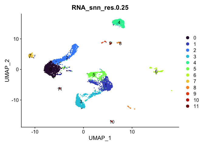
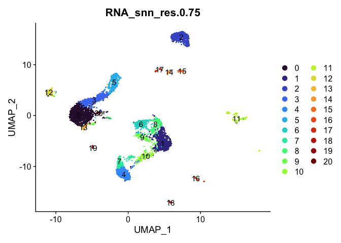
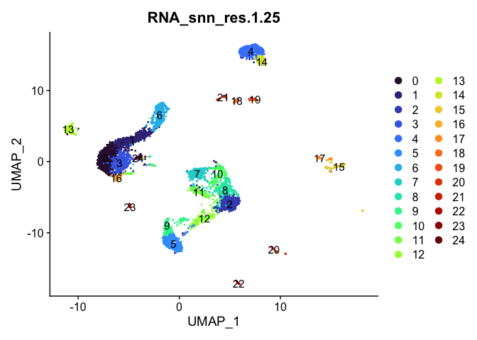
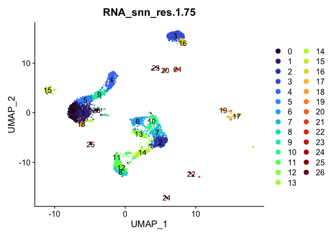
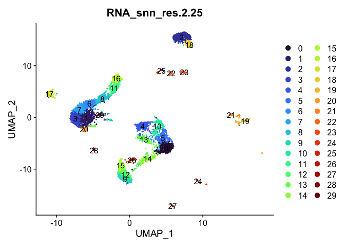
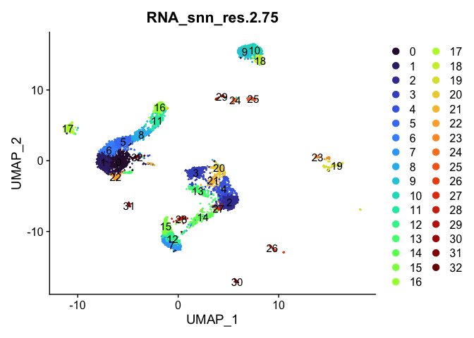
# UMAP colored by cluster
lapply(cluster.resolutions, function(res){
  DimPlot(experiment.aggregate,
          group.by = res,
          reduction = "umap",
          label = TRUE,
          shuffle = TRUE) +
    scale_color_viridis_d(option = "turbo")
})
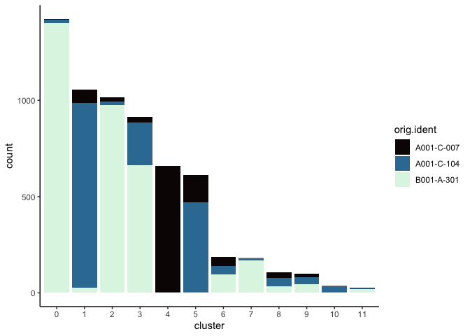
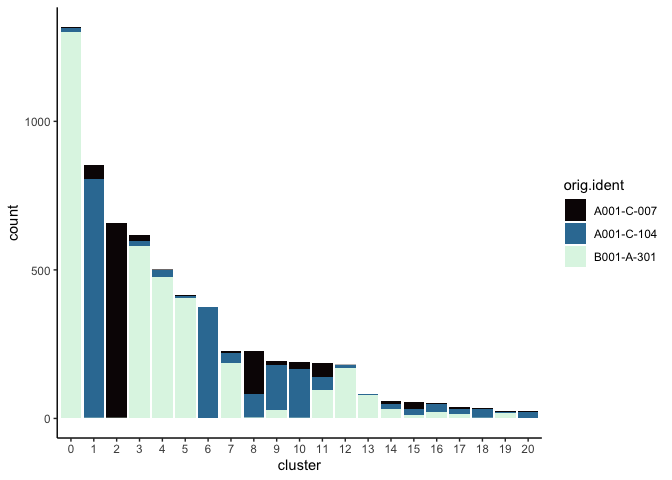
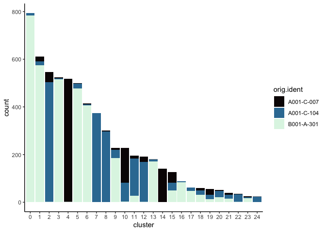
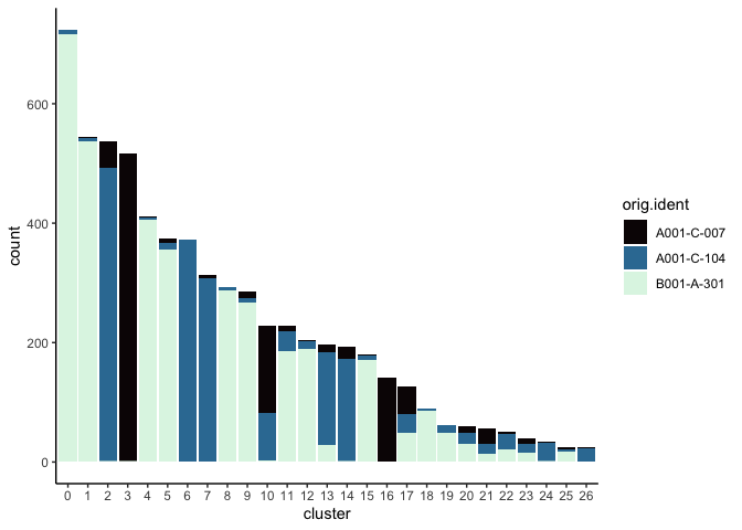
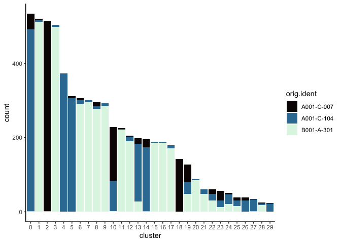
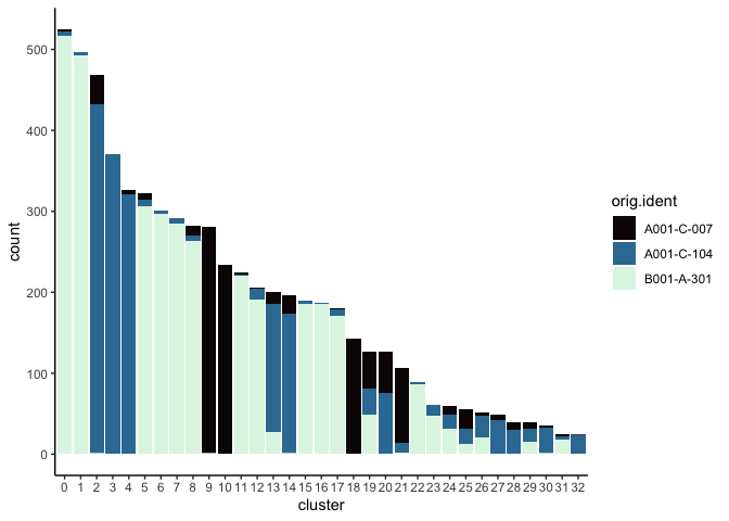
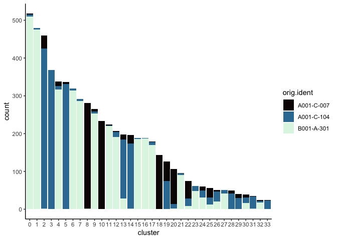
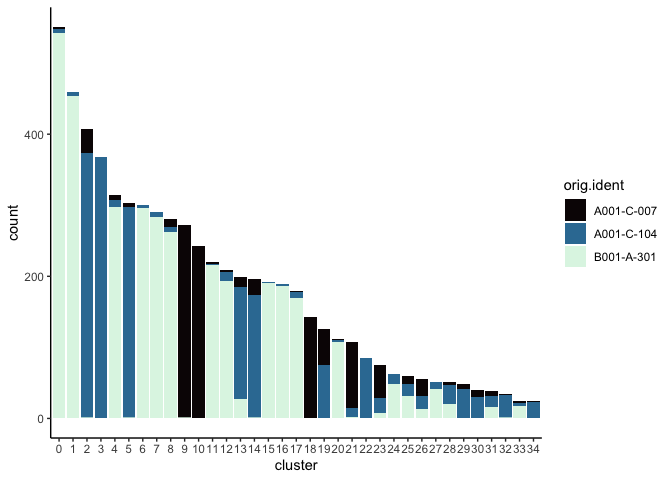
Investigate the relationship between cluster identity and sample identity
lapply(cluster.resolutions, function(res){
         tmp = experiment.aggregate@meta.data[,c(res, "orig.ident")]
         colnames(tmp) = c("cluster", "orig.ident")
         ggplot(tmp, aes(x = cluster, fill = orig.ident)) +
           geom_bar() +
           scale_fill_viridis_d(option = "mako") +
           theme_classic()
})
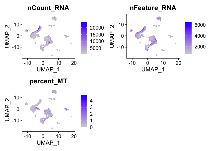
Visualize metadata
FeaturePlot(experiment.aggregate,
            reduction = "umap",
            features = c("nCount_RNA", "nFeature_RNA", "percent_MT"))
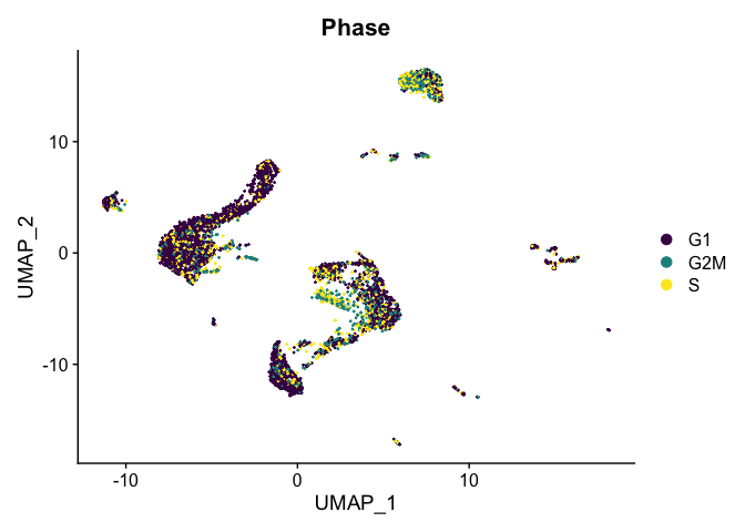
Visualize cell cycle phase
DimPlot(experiment.aggregate,
        reduction = "umap",
        group.by = "Phase",
        shuffle = TRUE) +
  scale_color_viridis_d()
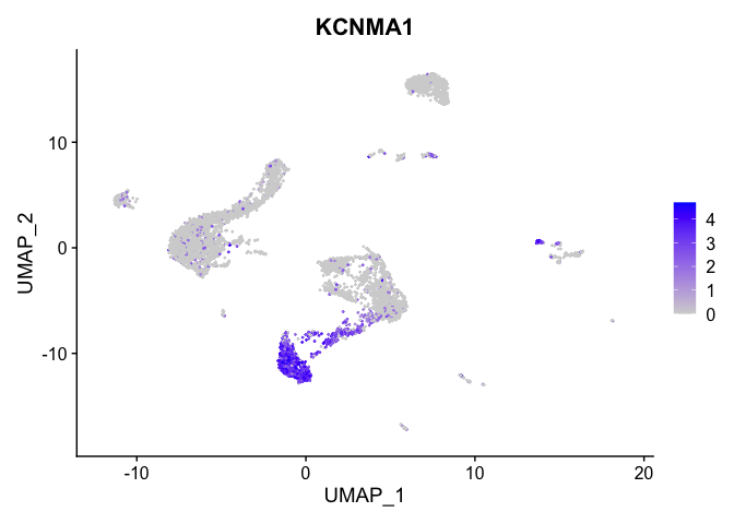
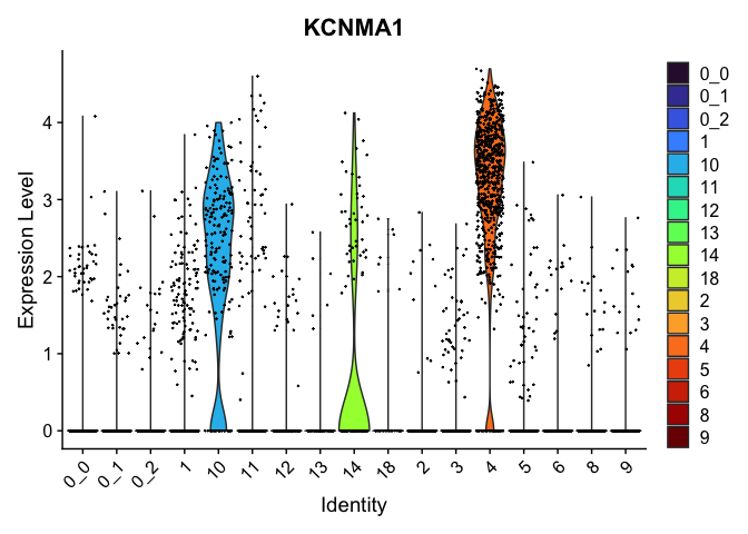
Visualize expression of genes of interest
FeaturePlot(experiment.aggregate,
            reduction = "umap",
            features = "KCNMA1")
Select a resolution
For now, let’s use resolution 0.75. Over the remainder of this section, we will refine the clustering further.
Idents(experiment.aggregate) <- "RNA_snn_res.0.75"
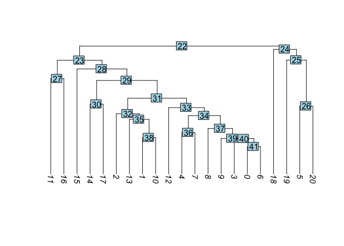
Visualize cluster tree
Building a phylogenetic tree relating the ‘average’ cell from each group in default ‘Ident’ (currently “RNA_snn_res.1.25”). Tree is estimated based on a distance matrix constructed in either gene expression space or PCA space.
experiment.aggregate <- BuildClusterTree(experiment.aggregate, dims = use.pcs)
PlotClusterTree(experiment.aggregate)
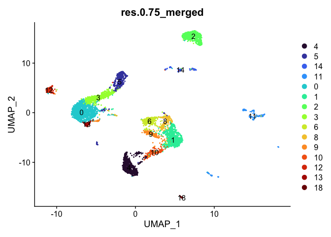
Merge clusters
In many experiments, the clustering resolution does not need to be uniform across all of the cell types present. While for some cell types of interest fine detail may be desirable, for others, simply grouping them into a larger parent cluster is sufficient. Merging cluster is very straightforward.
experiment.aggregate <- RenameIdents(experiment.aggregate,
                                     '7' = '4',
                                     '19' = '5',
                                     '20' = '5',
                                     '17' = '14',
                                     '15' = '14',
                                     '16' = '11')
experiment.aggregate$res.0.75_merged <- Idents(experiment.aggregate)
table(experiment.aggregate$res.0.75_merged)
DimPlot(experiment.aggregate,
        reduction = "umap",
        group.by = "res.0.75_merged",
        label = TRUE) +
  scale_color_viridis_d(option = "turbo")
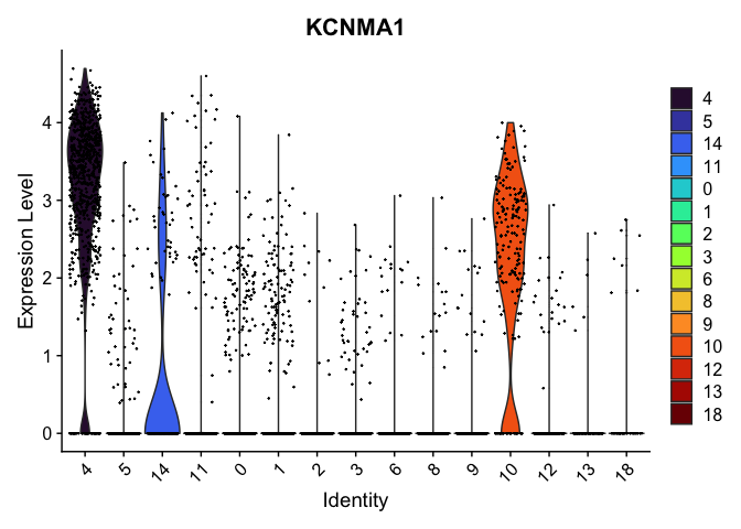
VlnPlot(experiment.aggregate,
        group.by = "res.0.75_merged",
        features = "KCNMA1") +
  scale_fill_viridis_d(option = "turbo")
Reorder the clusters
Merging the clusters changed the order in which they appear on a plot. In order to reorder the clusters for plotting purposes take a look at the levels of the identity, then re-level as desired.
levels(experiment.aggregate$res.0.75_merged)
# move one cluster to the first position
experiment.aggregate$res.0.75_merged <- relevel(experiment.aggregate$res.0.75_merged, "0")
levels(experiment.aggregate$res.0.75_merged)
# the color assigned to some clusters will change
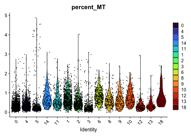
VlnPlot(experiment.aggregate,
group.by = "res.0.75_merged",
features = "percent_MT") +
scale_fill_viridis_d(option = "turbo")
# re-level entire factor
new.order <- as.character(sort(as.numeric(levels(experiment.aggregate$res.0.75_merged))))
experiment.aggregate$res.0.75_merged <- factor(experiment.aggregate$res.0.75_merged, levels = new.order)
levels(experiment.aggregate$res.0.75_merged)
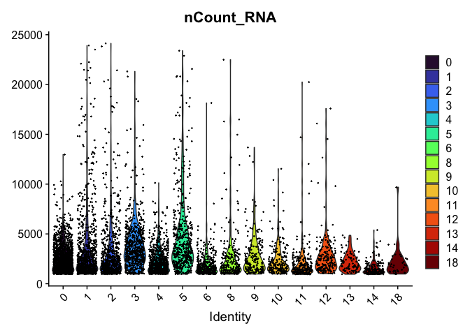
VlnPlot(experiment.aggregate,
        group.by = "res.0.75_merged",
        features = "nCount_RNA") +
  scale_fill_viridis_d(option = "turbo")
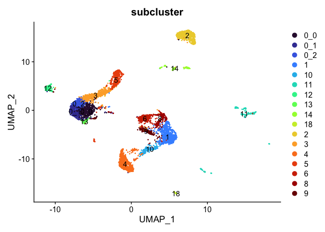
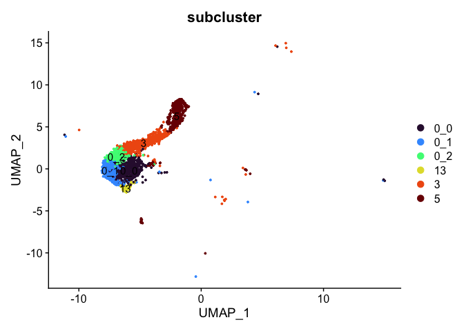
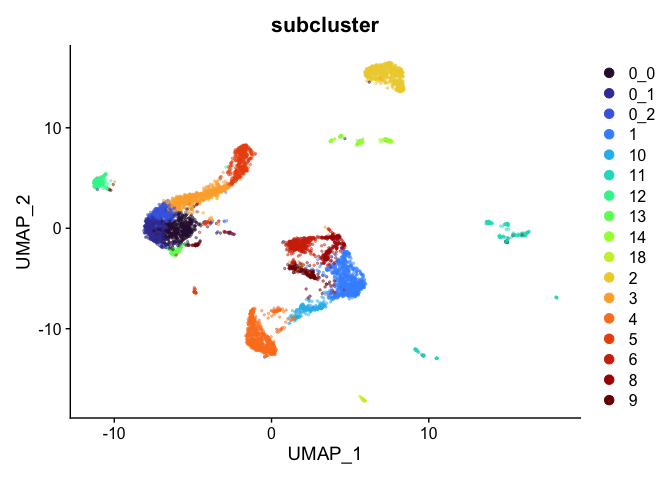
Subcluster
While merging clusters reduces the resolution in some parts of the experiment, sub-clustering has the opposite effect. Let’s produce sub-clusters for cluster 0.
experiment.aggregate <- FindSubCluster(experiment.aggregate,
                                       graph.name = "RNA_snn",
                                       cluster = 0,
                                       subcluster.name = "subcluster")
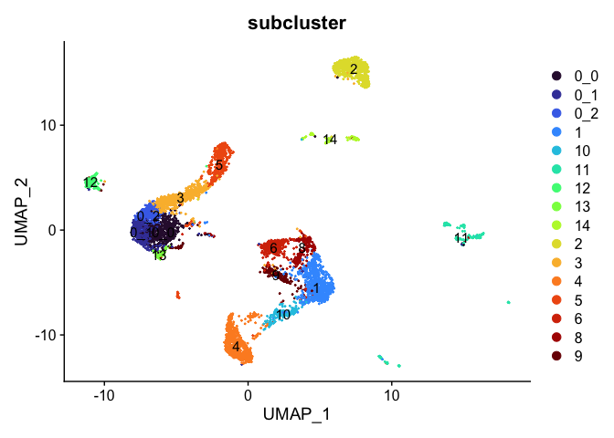
DimPlot(experiment.aggregate,
        reduction = "umap",
        group.by = "subcluster",
        label = TRUE,
        shuffle = TRUE) +
  scale_color_viridis_d(option = "turbo")
Sub-setting experiment by cluster identity
After exploring and refining the cluster resolution, we may have identified some clusters that are composed of cells we aren’t interested in. For example, if we have identified a cluster likely composed of contaminants, this cluster can be removed from the analysis. Alternatively, if a group of clusters have been identified as particularly of interest, these can be isolated and re-analyzed.
# remove cluster 18
Idents(experiment.aggregate) <- experiment.aggregate$subcluster
experiment.tmp <- subset(experiment.aggregate, subcluster != "18")
DimPlot(experiment.tmp,
        reduction = "umap",
        group.by = "subcluster",
        label = TRUE,
        shuffle = TRUE) +
  scale_color_viridis_d(option = "turbo")
# retain clusters 0_0, 0_1, 0_2, 3, 5, and 13
experiment.tmp <- subset(experiment.aggregate, subcluster %in% c("0_0", "0_1", "0_2", "3", "5", "13"))
DimPlot(experiment.tmp,
        reduction = "umap",
        group.by = "subcluster",
        label = TRUE,
        shuffle = TRUE) +
  scale_color_viridis_d(option = "turbo")
rm(experiment.tmp)
Identify marker genes
Seurat provides several functions that can help you find markers that define clusters via differential expression:
-
FindMarkersidentifies markers for a cluster relative to all other clusters -
FindAllMarkersperforms the find markers operation for all clusters -
FindAllMarkersNodedefines all markers that split a node from the cluster tree
FindMarkers
markers <- FindMarkers(experiment.aggregate,
                       group.by = "subcluster",
                       ident.1 = "0_2",
                       ident.2 = c("0_0", "0_1"))
length(which(markers$p_val_adj < 0.05)) # how many are significant?
head(markers) %>%
  kable() %>%
  kable_styling("striped")
| p_val | avg_log2FC | pct.1 | pct.2 | p_val_adj | |
|---|---|---|---|---|---|
| PPARGC1A | 0 | 0.8574109 | 0.885 | 0.572 | 0 |
| TRPM6 | 0 | 0.8593728 | 0.446 | 0.149 | 0 |
| PDE3A | 0 | 0.5157900 | 0.978 | 0.923 | 0 |
| CNNM2 | 0 | 0.7380028 | 0.849 | 0.505 | 0 |
| PARM1 | 0 | 0.7124092 | 0.756 | 0.388 | 0 |
| MICAL2 | 0 | 0.6546806 | 0.692 | 0.328 | 0 |
The “pct.1” and “pct.2” columns record the proportion of cells with normalized expression above 0 in ident.1 and ident.2, respectively. The “p_val” is the raw p-value associated with the differential expression test, while the BH-adjusted value is found in “p_val_adj”. Finally, “avg_logFC” is the average log fold change difference between the two groups.
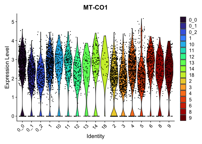
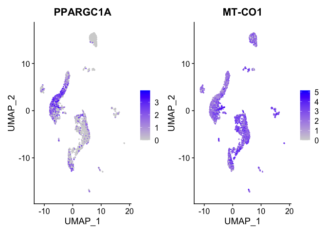
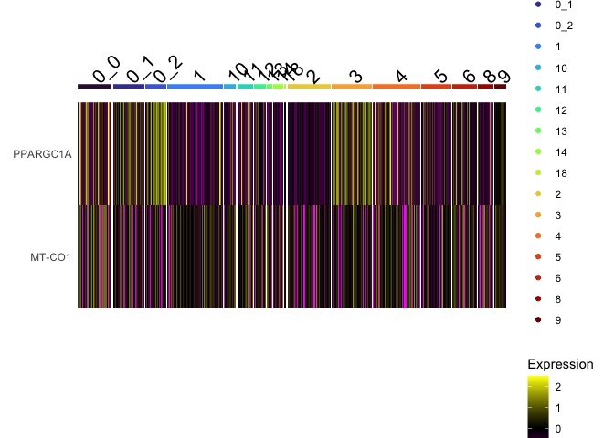
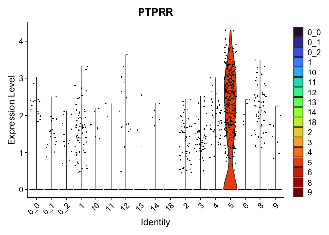
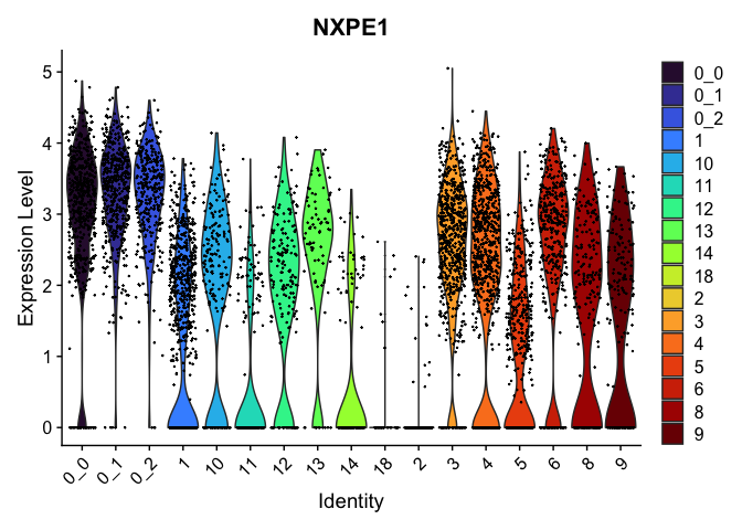
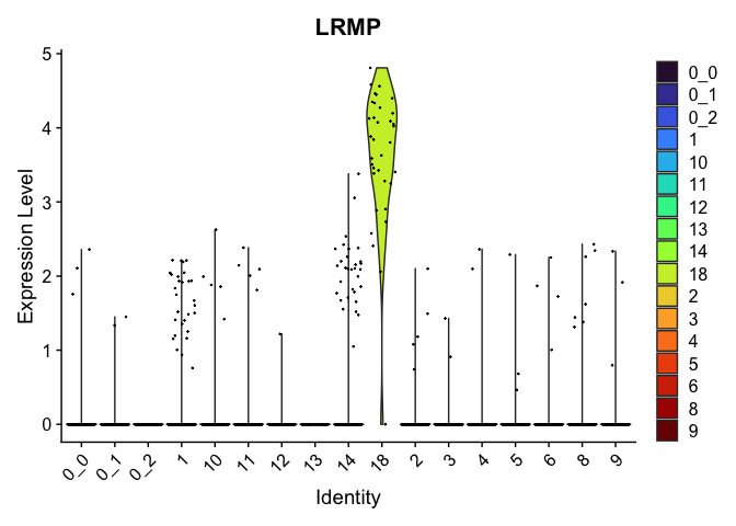
Marker genes identified this way can be visualized in violin plots, feature plots, and heat maps.
view.markers <- c(rownames(markers[markers$avg_log2FC > 0,])[1],
                  rownames(markers[markers$avg_log2FC < 0,])[1])
lapply(view.markers, function(marker){
  VlnPlot(experiment.aggregate,
          group.by = "subcluster",
          features = marker) +
    scale_fill_viridis_d(option = "turbo")
})

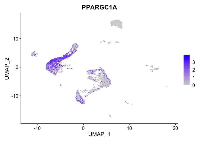
FeaturePlot(experiment.aggregate,
            features = view.markers,
            ncol = 2)
DoHeatmap(experiment.aggregate,
          group.by = "subcluster",
          features = view.markers,
          group.colors = viridis::turbo(length(unique(experiment.aggregate$subcluster))))
FindAllMarkers
FindAllMarkers can be used to automate this process across all genes.
markers <- FindAllMarkers(experiment.aggregate,
                          only.pos = TRUE,
                          min.pct = 0.25,
                          thresh.use = 0.25)
tapply(markers$p_val_adj, markers$cluster, function(x){
  length(x < 0.05)
})
head(markers) %>%
  kable() %>%
  kable_styling("striped")
| p_val | avg_log2FC | pct.1 | pct.2 | p_val_adj | cluster | gene | |
|---|---|---|---|---|---|---|---|
| LINC00278 | 0 | 1.825056 | 0.590 | 0.163 | 0 | 8 | LINC00278 |
| XAF1 | 0 | 1.532780 | 0.449 | 0.117 | 0 | 8 | XAF1 |
| DST | 0 | 1.681989 | 0.885 | 0.652 | 0 | 8 | DST |
| DUOX2 | 0 | 1.914879 | 0.322 | 0.068 | 0 | 8 | DUOX2 |
| CEACAM5 | 0 | 1.211420 | 0.855 | 0.514 | 0 | 8 | CEACAM5 |
| XDH | 0 | 2.047630 | 0.515 | 0.207 | 0 | 8 | XDH |
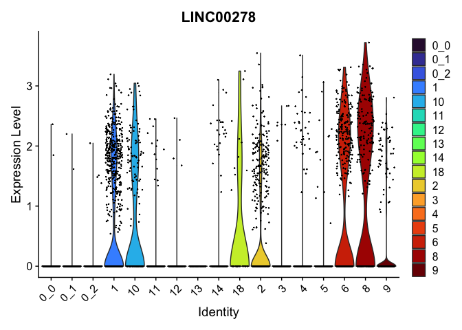
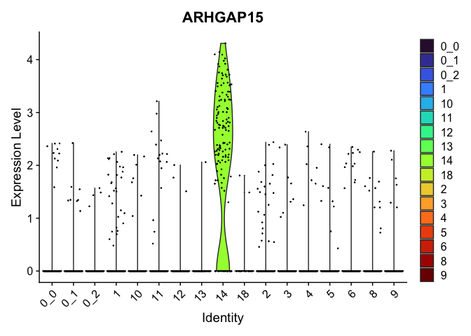
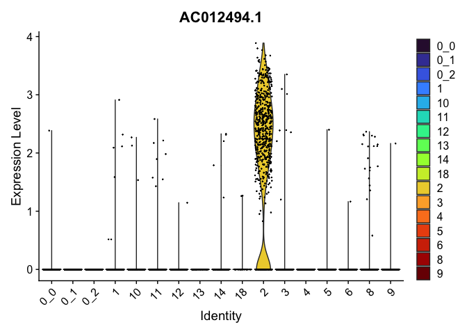
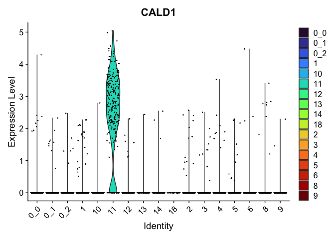
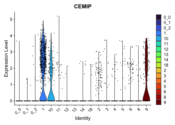
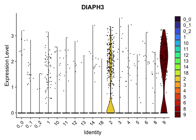
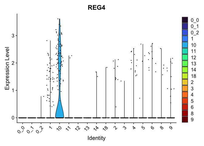
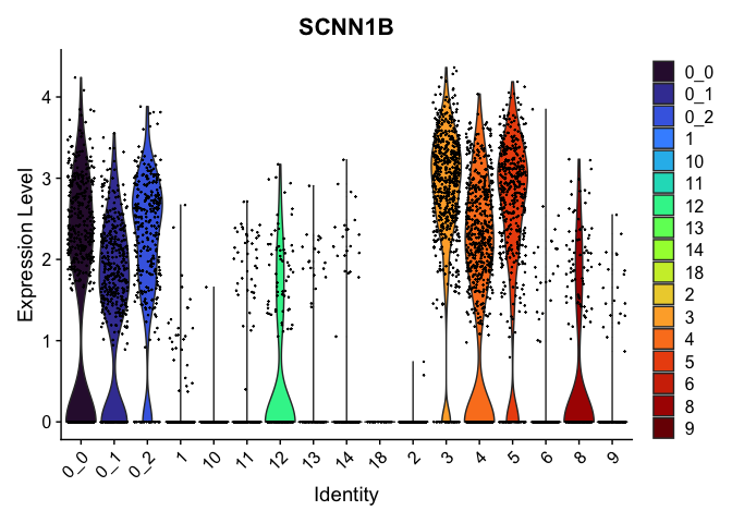
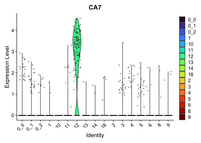
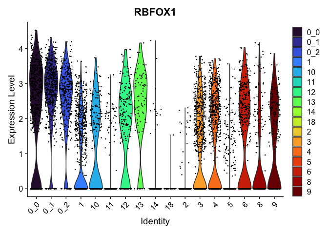
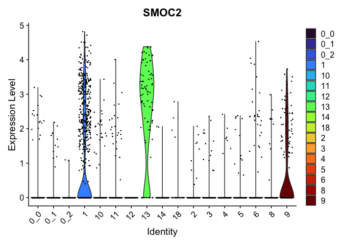
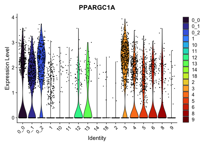
view.markers <- tapply(markers$gene, markers$cluster, function(x){head(x,1)})
# violin plots
lapply(view.markers, function(marker){
  VlnPlot(experiment.aggregate,
          group.by = "subcluster",
          features = marker) +
    scale_fill_viridis_d(option = "turbo")
})

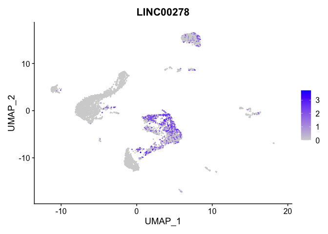
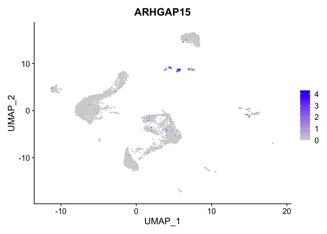
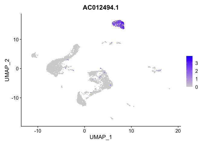
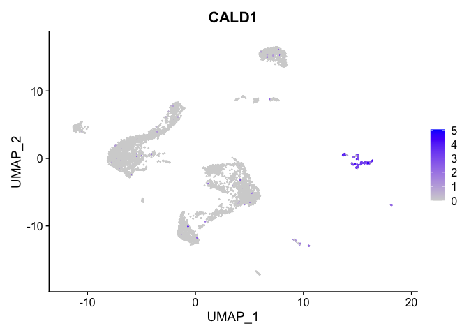
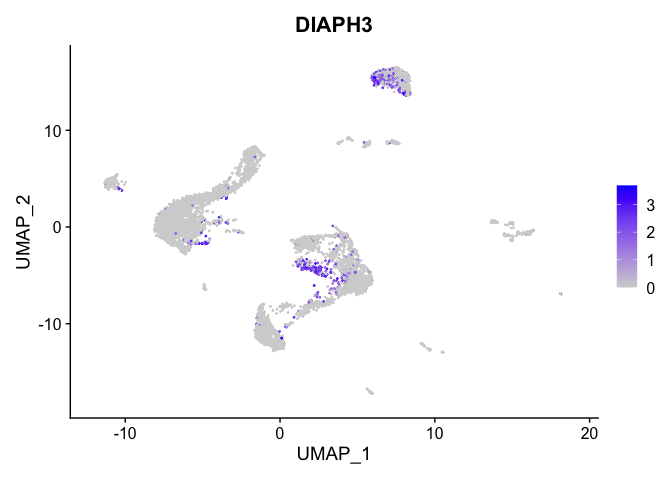
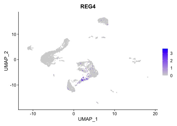
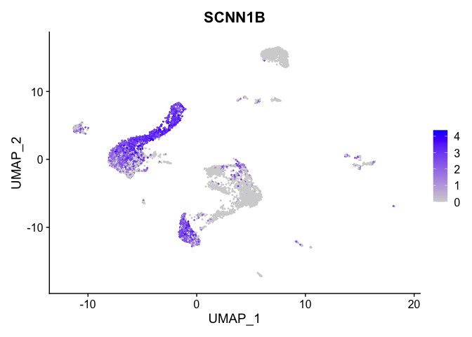
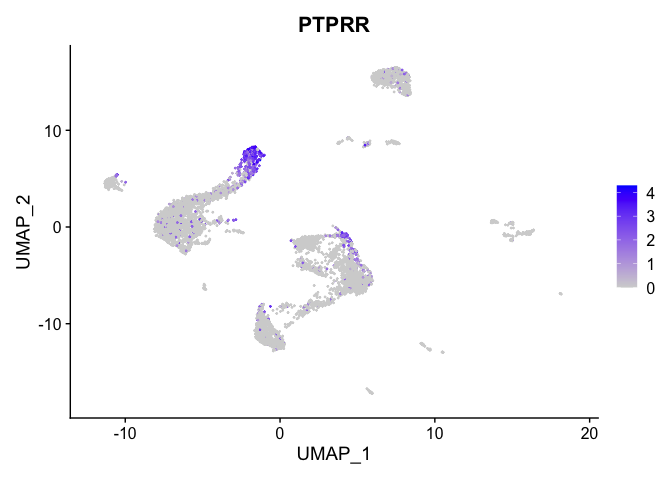
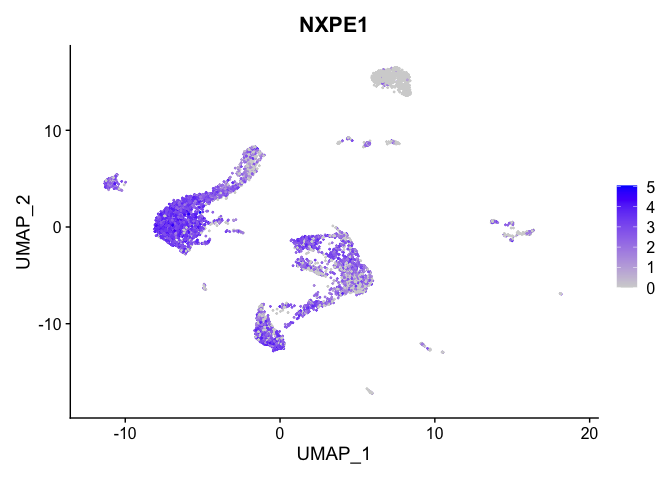
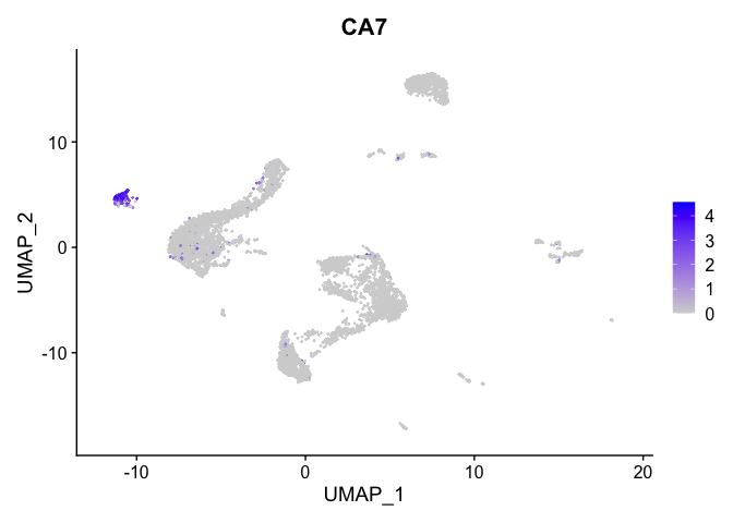
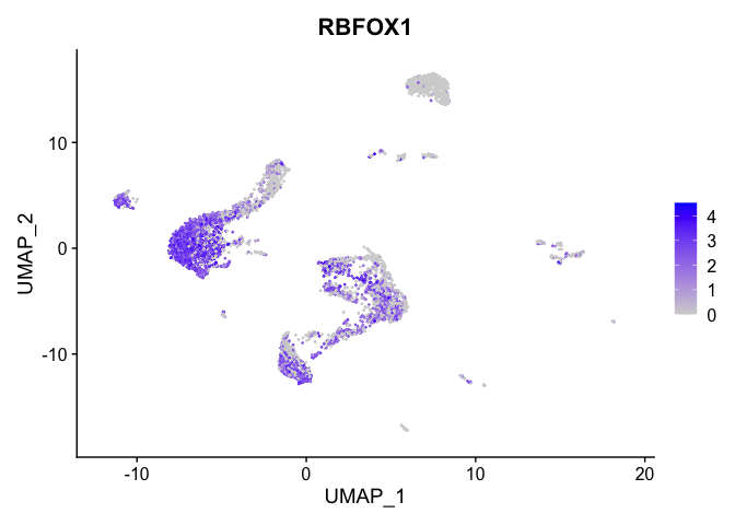
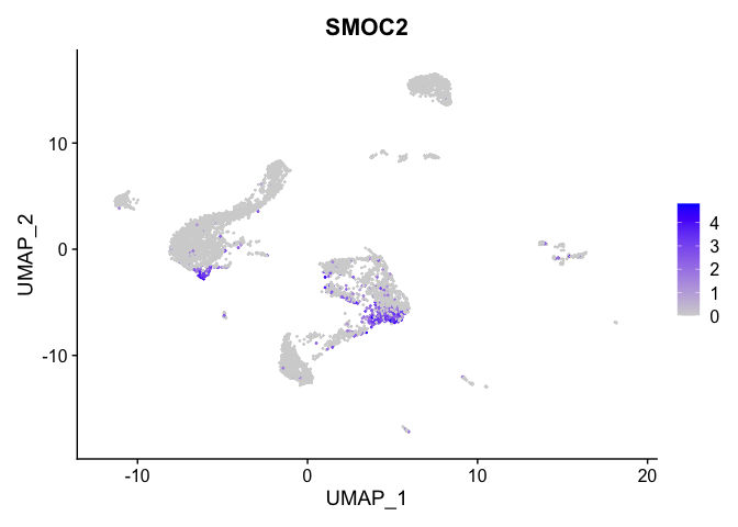
# feature plots
lapply(view.markers, function(marker){
  FeaturePlot(experiment.aggregate,
              features = marker)
})


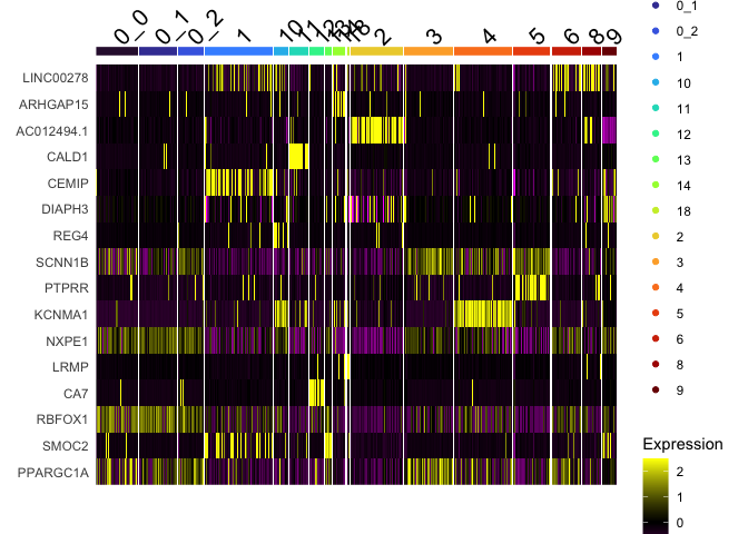
# heat map
DoHeatmap(experiment.aggregate,
          group.by = "subcluster",
          features = view.markers,
          group.colors = viridis::turbo(length(unique(experiment.aggregate$subcluster))))
Calculate mean marker expression within clusters
You may want to get an idea of the mean expression of markers in a cluster or group of clusters. The percent expressing is provided by FindMarkers and FindAllMarkers, along with the average log fold change, but not the expression value itself. The function below calculates a mean for the supplied marker in the named cluster(s) and all other groups. Please note that this function accesses the active identity.
# ensure active identity is set to desired clustering resolution
Idents(experiment.aggregate) <- experiment.aggregate$subcluster
# define function
getGeneClusterMeans <- function(feature, idents){
  x = GetAssayData(experiment.aggregate)[feature,]
  m = tapply(x, Idents(experiment.aggregate) %in% idents, mean)
  names(m) = c("mean.out.of.idents", "mean.in.idents")
  return(m[c(2,1)])
}
# calculate means for a single marker
getGeneClusterMeans("SMOC2", c("1"))
# add means to marker table (example using subset)
markers.small <- markers[view.markers,]
means <- matrix(mapply(getGeneClusterMeans, view.markers, markers.small$cluster), ncol = 2, byrow = TRUE)
colnames(means) <- c("mean.in.cluster", "mean.out.of.cluster")
rownames(means) <- view.markers
markers.small <- cbind(markers.small, means)
markers.small[,c("cluster", "mean.in.cluster", "mean.out.of.cluster", "avg_log2FC", "p_val_adj")] %>%
  kable() %>%
  kable_styling("striped")
| cluster | mean.in.cluster | mean.out.of.cluster | avg_log2FC | p_val_adj | |
|---|---|---|---|---|---|
| LINC00278 | 8 | 1.3905765 | 0.3126136 | 1.8250560 | 0 |
| ARHGAP15 | 14 | 2.0999714 | 0.0420769 | 3.8168553 | 0 |
| AC012494.1 | 2 | 1.9829173 | 0.0198549 | 3.4055733 | 0 |
| CALD1 | 11 | 2.4889292 | 0.0321684 | 4.2588299 | 0 |
| CEMIP | 1 | 1.7103302 | 0.1470160 | 2.9158868 | 0 |
| DIAPH3 | 2 | 0.7078035 | 0.1208302 | 1.3733030 | 0 |
| REG4 | 10 | 0.8891786 | 0.0282499 | 2.2188514 | 0 |
| SCNN1B | 3 | 2.7606983 | 0.8929028 | 1.9172739 | 0 |
| PTPRR | 5 | 1.7170380 | 0.1082672 | 2.9851173 | 0 |
| KCNMA1 | 10 | 2.1932315 | 0.5296899 | 1.4143155 | 0 |
| NXPE1 | 3 | 2.5301263 | 1.7681133 | 0.3819432 | 0 |
| LRMP | 18 | 3.6264698 | 0.0292279 | 5.4904492 | 0 |
| CA7 | 12 | 2.7331103 | 0.0397866 | 4.5913220 | 0 |
| LINC00278.1 | 8 | 1.3905765 | 0.3126136 | 1.8250560 | 0 |
| RBFOX1 | 0_0 | 2.1639139 | 1.1637186 | 1.2089765 | 0 |
| SMOC2 | 1 | 1.0332466 | 0.1219120 | 2.2988903 | 0 |
| PPARGC1A | 3 | 2.0532474 | 0.6728933 | 1.6622156 | 0 |
Advanced visualizations
Researchers may use the tree, markers, domain knowledge, and goals to identify useful clusters. This may mean adjusting PCA to use, choosing a new resolution, merging clusters together, sub-clustering, sub-setting, etc. You may also want to use automated cell type identification at this point, which will be discussed in the next section.
Address overplotting
Single cell and single nucleus experiments may include so many cells that dimensionality reduction plots sometimes suffer from overplotting, where individual points are difficult to see. The following code addresses this by adjusting the size and opacity of the points.
alpha.use <- 0.4
p <- DimPlot(experiment.aggregate,
             group.by="subcluster",
             pt.size=0.5,
             reduction = "umap",
             shuffle = TRUE) +
  scale_color_viridis_d(option = "turbo")
p$layers[[1]]$mapping$alpha <- alpha.use
p + scale_alpha_continuous(range = alpha.use, guide = FALSE)
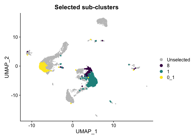
Highlight a subset
DimPlot(experiment.aggregate,
        group.by = "subcluster",
        cells.highlight = CellsByIdentities(experiment.aggregate, idents = c("0_1", "8", "1")),
        cols.highlight = c(viridis::viridis(3))) +
  ggtitle("Selected sub-clusters")
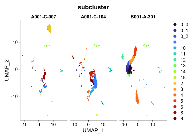
Split dimensionality reduction plots
DimPlot(experiment.aggregate,
        group.by = "subcluster",
        split.by = "orig.ident") +
  scale_color_viridis_d(option = "turbo")
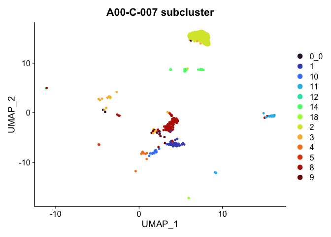
Plot a subset of cells
Note that the object itself is unchanged by the subsetting operation.
DimPlot(experiment.aggregate,
        group.by = "subcluster",
        reduction = "umap",
        cells = Cells(experiment.aggregate)[experiment.aggregate$orig.ident %in% "A001-C-007"]) +
  scale_color_viridis_d(option = "turbo") +
  ggtitle("A00-C-007 subcluster")
Save the Seurat object and download the next Rmd file
# set the finalcluster to subcluster
experiment.aggregate$finalcluster <- experiment.aggregate$subcluster
# save object
saveRDS(experiment.aggregate, file="scRNA_workshop_4.rds")
download.file("https://raw.githubusercontent.com/ucdavis-bioinformatics-training/2023-June-Single-Cell-RNA-Seq-Analysis/main/data_analysis/scRNA_Workshop-PART5.Rmd", "scRNA_Workshop-PART5.Rmd")
Session Information
sessionInfo()