☰ Menu

      Single Cell RNA-Seq Analysis

Home
Introduction and Lectures
Intro to the Workshop and Core
Schedule
What is Bioinformatics/Genomics?
Experimental Design and Cost Estimation
Support
Slack
Zoom
Cheat Sheets
Software and Links
Scripts
Prerequisites
CLI
R
Data Reduction
Files and Filetypes
Project setup
Generating Expression Matrix
scRNAseq Analysis
Prepare scRNAseq Analysis
scRNAseq Analysis - PART1
scRNAseq Analysis - PART2
scRNAseq Analysis - PART3
scRNAseq Analysis - PART4
scRNAseq Analysis - PART5
scRNAseq Analysis - PART6
scRNAseq Analysis - PART7
ETC
Closing thoughts
Workshop Photos
Github page
Biocore website

Part 5: Enrichment, Model-Based DE, and Cell-Type Identification

Load libraries

library(Seurat)
library(limma)
library(topGO)
library(HGNChelper)
library(dplyr)

Load the Seurat object

experiment.merged <- readRDS("scRNA_workshop_4.rds")
experiment.merged
An object of class Seurat 11292 features across 6312 samples within 1 assay Active assay: RNA (11292 features, 7012 variable features) 3 dimensional reductions calculated: pca, tsne, umap
Idents(experiment.merged) <- "finalcluster"

1. Gene Ontology (GO) Enrichment of Genes Expressed in a Cluster

Gene Ontology provides a controlled vocabulary for describing gene products. Here we use enrichment analysis to identify GO terms that are overrepresented among the gene expressed in cells in a given cluster.

cluster10 <- subset(experiment.merged, idents = '10')
expr <- as.matrix(GetAssayData(cluster10))

# Select genes that are expressed > 0 in at least half of cells
n.gt.0 <- apply(expr, 1, function(x)length(which(x > 0)))
expressed.genes <- rownames(expr)[which(n.gt.0/ncol(expr) >= 0.5)]
all.genes <- rownames(expr)

# define geneList as 1 if gene is in expressed.genes, 0 otherwise
geneList <- ifelse(all.genes %in% expressed.genes, 1, 0)
names(geneList) <- all.genes

# Create topGOdata object
	GOdata <- new("topGOdata",
		ontology = "BP", # use biological process ontology
		allGenes = geneList,
		geneSelectionFun = function(x)(x == 1),
              annot = annFUN.org, mapping = "org.Hs.eg.db", ID = "symbol")
# Test for enrichment using Fisher's Exact Test
	resultFisher <- runTest(GOdata, algorithm = "elim", statistic = "fisher")
	GenTable(GOdata, Fisher = resultFisher, topNodes = 20, numChar = 60)
GO.ID Term Annotated Significant Expected Fisher 1 GO:0030644 intracellular chloride ion homeostasis 8 4 0.32 0.00015 2 GO:0030050 vesicle transport along actin filament 15 5 0.59 0.00020 3 GO:0030036 actin cytoskeleton organization 462 40 18.19 0.00020 4 GO:0051660 establishment of centrosome localization 9 4 0.35 0.00025 5 GO:0006895 Golgi to endosome transport 17 5 0.67 0.00039 6 GO:0045053 protein retention in Golgi apparatus 5 3 0.20 0.00057 7 GO:0032534 regulation of microvillus assembly 5 3 0.20 0.00057 8 GO:0043268 positive regulation of potassium ion transport 19 5 0.75 0.00068 9 GO:0035176 social behavior 19 5 0.75 0.00068 10 GO:0009653 anatomical structure morphogenesis 1495 96 58.87 0.00093 11 GO:0030155 regulation of cell adhesion 473 33 18.62 0.00096 12 GO:2000650 negative regulation of sodium ion transmembrane transporter ... 6 3 0.24 0.00111 13 GO:0000381 regulation of alternative mRNA splicing, via spliceosome 42 7 1.65 0.00114 14 GO:0090630 activation of GTPase activity 82 10 3.23 0.00135 15 GO:1904908 negative regulation of maintenance of mitotic sister chromat... 2 2 0.08 0.00155 16 GO:0048669 collateral sprouting in absence of injury 2 2 0.08 0.00155 17 GO:0042060 wound healing 262 21 10.32 0.00155 18 GO:0007163 establishment or maintenance of cell polarity 160 15 6.30 0.00158 19 GO:0045944 positive regulation of transcription by RNA polymerase II 791 48 31.15 0.00158 20 GO:0040018 positive regulation of multicellular organism growth 14 4 0.55 0.00173

Quiz 1

2. Model-based DE analysis in limma

limma is an R package for differential expression analysis of bulk RNASeq and microarray data. We apply it here to single cell data.

Limma can be used to fit any linear model to expression data and is useful for analyses that go beyond two-group comparisons. A detailed tutorial of model specification in limma is available here and in the limma User’s Guide.

# filter genes to those expressed in at least 10% of cells
keep <- rownames(expr)[which(n.gt.0/ncol(expr) >= 0.1)]
expr2 <- expr[keep,]

# Set up "design matrix" with statistical model
cluster10$proper.ident <- make.names(cluster10$orig.ident)
mm <- model.matrix(~0 + proper.ident + S.Score + G2M.Score + percent_MT + nFeature_RNA, data = cluster10[[]])
head(mm)
proper.identA001.C.007 proper.identA001.C.104 proper.identB001.A.301 S.Score G2M.Score percent_MT nFeature_RNA AAGCCATCAAGACCTT_A001-C-007 1 0 0 0.06496555 -0.07473751 0.4904632 1253 AAGTTCGGTACCTATG_A001-C-007 1 0 0 0.01208720 -0.03974145 0.5266623 1127 AATGAAGTCAGCGTCG_A001-C-007 1 0 0 0.11081470 0.07119225 1.0507881 1262 ACAGAAATCCAGCTCT_A001-C-007 1 0 0 -0.04751440 -0.06997775 0.6423123 1610 ACGGTTACAAATCGGG_A001-C-007 1 0 0 -0.02654739 0.13670266 0.7633588 1899 AGAGAGCGTTCTCCTG_A001-C-007 1 0 0 -0.08564181 0.36355846 0.3964321 780
tail(mm)
proper.identA001.C.007 proper.identA001.C.104 proper.identB001.A.301 S.Score G2M.Score percent_MT nFeature_RNA TTGCCTGTCCGCGATG_A001-C-104 0 1 0 -0.06933278 -0.02305915 0.3658218 2207 TTGGGATTCGTTCCCA_A001-C-104 0 1 0 -0.06606713 -0.09091689 0.4091653 1547 TTGTTTGCACTACGGC_A001-C-104 0 1 0 0.10614897 0.16666296 0.5232806 4131 TTTCAGTTCGCACTCT_A001-C-104 0 1 0 -0.09860144 -0.06928261 1.8292683 1291 TTTGTTGTCGAGATGG_A001-C-104 0 1 0 0.53662508 -0.01783252 1.1442709 3158 GACTCAACACACACGC_B001-A-301 0 0 1 0.05115791 -0.10329846 0.1606426 973
# Fit model in limma
fit <- lmFit(expr2, mm)
head(coef(fit))
proper.identA001.C.007 proper.identA001.C.104 proper.identB001.A.301 S.Score G2M.Score percent_MT nFeature_RNA C1orf159 0.09035597 0.05713314 -0.12377511 -0.04907108 0.2390908 0.0265014 1.507975e-04 SDF4 0.37198100 0.48933012 0.18564080 0.02277449 0.7557869 -0.2090015 -7.724535e-05 CCNL2 0.45862277 0.30595382 1.86485404 0.44929124 -0.6053252 0.1915253 2.435578e-04 MIB2 0.03562615 0.16762967 -0.09454838 -0.11151005 -0.4005421 -0.1667042 8.803433e-05 CDK11B 0.57768924 -0.17984772 -0.19687762 -0.61947055 0.1419469 0.2500343 2.087001e-04 SLC35E2B 0.03496575 0.07970405 -0.04265325 -0.38532142 0.2340181 0.1238448 6.849378e-05
# Test 'B001-A-301' - 'A001-C-007'
contr <- makeContrasts(proper.identB001.A.301 - proper.identA001.C.007, levels = colnames(coef(fit)))
fit2 <- contrasts.fit(fit, contrasts = contr)
fit2 <- eBayes(fit2)
out <- topTable(fit2, n = Inf, sort.by = "P")
head(out, 30)
logFC AveExpr t P.Value adj.P.Val B UTP6 2.771737 0.1647313 5.555220 9.135633e-08 0.0004364092 7.4033275 S100PBP 2.812186 0.2142075 5.015554 1.197360e-06 0.0028598939 5.0912200 ALG14 2.210138 0.1503340 4.767290 3.675731e-06 0.0048251558 4.0869951 ZNF525 2.425630 0.1652124 4.745937 4.040323e-06 0.0048251558 4.0024512 TXNL4A 2.089932 0.1416849 4.628829 6.750082e-06 0.0064490285 3.5440387 CMSS1 2.166560 0.1630744 4.398707 1.800823e-05 0.0114155254 2.6696461 FAM204A 2.180902 0.1590753 4.371382 2.018435e-05 0.0114155254 2.5681911 WDTC1 2.198629 0.1694821 4.332526 2.371794e-05 0.0114155254 2.4247952 ADAMTSL1 3.418667 0.4165572 4.315208 2.547738e-05 0.0114155254 2.3612183 NMRAL1 2.292548 0.1813030 4.307704 2.627798e-05 0.0114155254 2.3337349 TCP11L1 2.202365 0.1649595 4.307625 2.628654e-05 0.0114155254 2.3334459 ZNF43 2.319958 0.1859967 4.205410 3.990650e-05 0.0158861114 1.9629628 LNX2 2.752712 0.2984931 4.156446 4.861261e-05 0.0174846771 1.7880754 KLHL36 2.021210 0.1583305 4.128697 5.432365e-05 0.0174846771 1.6897099 PROX1 2.292479 0.1760185 4.104031 5.993316e-05 0.0174846771 1.6027298 CRKL 2.137632 0.1798690 4.095706 6.194832e-05 0.0174846771 1.5734680 ZNF3 2.254016 0.1913725 4.079704 6.600427e-05 0.0174846771 1.5173672 IRF3 2.718407 0.3001289 4.060982 7.107132e-05 0.0174846771 1.4519605 CDK18 2.162366 0.1708365 4.060577 7.118518e-05 0.0174846771 1.4505452 RXRA 2.056970 0.1731630 4.050718 7.400472e-05 0.0174846771 1.4162056 MED17 2.159188 0.1828195 4.041080 7.686377e-05 0.0174846771 1.3827025 TTC7A 2.201710 0.1728635 4.026694 8.132775e-05 0.0176592125 1.3328189 ZNF480 2.271793 0.2030146 4.011207 8.640911e-05 0.0179467969 1.2792824 RBL1 2.208890 0.2095978 3.971884 1.007047e-04 0.0200444376 1.1441201 SARS 2.384320 0.2063039 3.945727 1.114307e-04 0.0209300889 1.0548315 NFU1 1.973533 0.1593605 3.940006 1.139172e-04 0.0209300889 1.0353696 RAB22A 2.100397 0.2068305 3.914924 1.254551e-04 0.0221962542 0.9503174 PPIL4 2.205829 0.2056979 3.895878 1.349488e-04 0.0230232310 0.8860400 ADPGK 2.013676 0.1634801 3.881872 1.423612e-04 0.0234503229 0.8389417 RNF13 2.170378 0.1892707 3.850945 1.601209e-04 0.0249376083 0.7354474

Output columns:

Quiz 2

Cell type identification with ScType

ScType assigns our clusters from Seurat to a cell type based on a hierarchical external database.

The database supplied with the package is human but users can supply their own data.

More details are available on Github:

Source ScType functions from Github:

# load gene set preparation function
source("https://raw.githubusercontent.com/IanevskiAleksandr/sc-type/master/R/gene_sets_prepare.R")
# load cell type annotation function
source("https://raw.githubusercontent.com/IanevskiAleksandr/sc-type/master/R/sctype_score_.R")

Read in marker database:

# DB file
db_ = "https://raw.githubusercontent.com/IanevskiAleksandr/sc-type/master/ScTypeDB_full.xlsx";
tissue = "Intestine" # e.g. Immune system,Pancreas,Liver,Eye,Kidney,Brain,Lung,Adrenal,Heart,Intestine,Muscle,Placenta,Spleen,Stomach,Thymus 

# prepare gene sets
gs_list = gene_sets_prepare(db_, tissue)

Let’s take a look at the structure of the marker database:
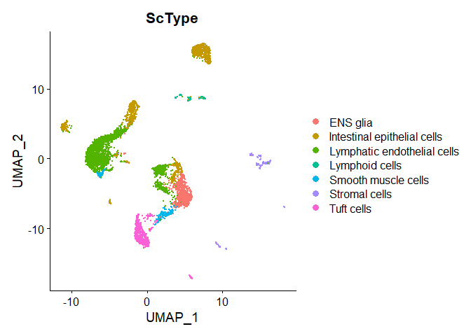
head(gs_list)
$gs_positive $gs_positive$Erythroblasts [1] "AHSP" "ALAS2" "GYPA" "HBA1" "HBA2" "HBB" "HBG1" "HBG2" "HBM" "HBZ" "HEMGN" "MIR144" "MYL4" "SLC4A1" "SPTA1" $gs_positive$`Chromaffin cells` [1] "ARX" "ASIC5" "CCK" "CRYBA2" "FEV" "KCNH6" "MLN" "NEUROD1" "NKX2-2" "ONECUT3" "PAX4" "PCSK1" "SST" "SSTR5" $gs_positive$`Smooth muscle cells` [1] "ACTG2" "ANO1" "CHRDL2" "CNN1" "DES" "FBXL22" "FRMD6-AS2" "GREM2" "MYH11" "OVCH2" "TACR2" "TAGLN" "WIF1" $gs_positive$`Myeloid cells` [1] "C1QB" "C1QC" "DCANP1" "CD163" "CD207" "DNASE1L3" "HCAR3" "IL1B" "LILRB2" "LILRB5" "P2RY13" "RPL32P1" "VSIG4" $gs_positive$`Lymphoid cells` [1] "CCR4" "CD247" "GZMA" "GZMK" "ICOS" "IL17A" "LTA" "NCR2" "SH2D1A" "TRDC" "TRGC1" "VPREB1" $gs_positive$`Intestinal epithelial cells` [1] "ALPI" "ARL14" "LEXM" "CA7" "DEFB1" "EGFR-AS1" "HMGN1P20" "LINC00955" "TRIM31" "UNC5CL" $gs_positive$`ENS glia` [1] "BCAN" "CDH19" "COL20A1" "FOXD3" "GPR12" "MPZ" "PLP1" "PTPRZ1" "RLBP1" "SERPINA3" "SOX10" "SOX2" "SOX2-OT" "TFAP2A" $gs_positive$`ENS neurons` [1] "CEND1" "DRGX" "GAL" "GCGR" "GRP" "HECW1-IT1" "IQCJ" "NEFL" "PDIA2" "PHOX2A" "SLC18A3" "STMN4" "TTC9B" $gs_positive$`Vascular endothelial cells` [1] "APLNR" "BTNL9" "CLEC3B" "ESAM" "ESM1" "FLT1" "GJA5" "GPIHBP1" "LHX6" "MMRN2" "NOTCH4" "PRND" "SOX17" $gs_positive$`Stromal cells` [1] "CXCL14" "FZD10" "ITGA11" "MMP27" "MSC" "PDGFRA" $gs_positive$`Mesothelial cells` [1] "BNC1" "C21orf62" "C3" "CEMP1" "CRB2" "DSC3" "HAS1" "KLK11" "PHYHIP" "PTPRQ" "TGM1" "TNNT1" "WNT10A" "WT1" $gs_positive$`Lymphatic endothelial cells` [1] "ABCA4" "ART5" "CCL21" "GPR1" "LINC00636" "MPP7" "PLIN5" "STAB2" "TBX1" "TP63" "TSPEAR" $gs_negative $gs_negative$Erythroblasts character(0) $gs_negative$`Chromaffin cells` character(0) $gs_negative$`Smooth muscle cells` character(0) $gs_negative$`Myeloid cells` character(0) $gs_negative$`Lymphoid cells` character(0) $gs_negative$`Intestinal epithelial cells` character(0) $gs_negative$`ENS glia` character(0) $gs_negative$`ENS neurons` character(0) $gs_negative$`Vascular endothelial cells` character(0) $gs_negative$`Stromal cells` character(0) $gs_negative$`Mesothelial cells` character(0) $gs_negative$`Lymphatic endothelial cells` character(0)

Let’s add a cell type and associated markers (markers from https://panglaodb.se/markers.html?cell_type=%27Tuft%20cells%27#google_vignette):

gs_list$gs_positive$`Tuft cells` <- c("SUCNR1", "FABP1", "POU2F3", "SIGLECF", "CDHR2", "AVIL", "ESPN", "LRMP", "TRPM5", "DCLK1", "TAS1R3", "SOX9", "TUBB5", "CAMK2B", "GNAT3", "IL25", "PLCB2", "GFI1B", "ATOH1", "CD24A", "ASIC5", "KLF3", "KLF6", "DRD3", "NRADD", "GNG13", "NREP", "RGS2", "RAC2", "PTGS1", "IRF7", "FFAR3", "ALOX5", "TSLP", "IL4RA", "IL13RA1", "IL17RB", "PTPRC")
gs_list$gs_negative$`Tuft cells` <- NULL
# get cell-type by cell matrix
scale.data <- GetAssayData(experiment.merged, "scale")
es.max = sctype_score(scRNAseqData = scale.data, scaled = TRUE, 
                      gs = gs_list$gs_positive, gs2 = gs_list$gs_negative) 
# cell type scores for first cell
es.max[,1]
Smooth muscle cells Lymphoid cells Intestinal epithelial cells ENS glia Vascular endothelial cells Stromal cells Lymphatic endothelial cells Tuft cells -0.3240119 -0.1071450 -0.4512850 -0.1365531 -0.1035601 -0.1551877 2.1424191 0.6259383

We will derive a cluster-level score by summing the cell level scores within each cluster

tmp <- lapply(sort(unique(experiment.merged$finalcluster)), function(cl, nkeep = 3){
  es.max.cl <- sort(rowSums(es.max[, experiment.merged$finalcluster == cl]), decreasing = TRUE)
  out <- head(data.frame(finalcluster = cl, ScType = names(es.max.cl), scores = es.max.cl, ncells = sum(experiment.merged$finalcluster == cl)), nkeep)
  out$rank <- 1:nkeep
  return(out)
})
cL_results.top <- do.call("rbind", tmp)
cL_results.top1 <- subset(cL_results.top, rank == 1)

Merge ScType cluster-level results with Seurat object

tmp <- data.frame(cell = colnames(experiment.merged), finalcluster = experiment.merged$finalcluster)
tmp <- left_join(tmp, cL_results.top1, by = "finalcluster")
experiment.merged$ScType <- tmp$ScType
DimPlot(experiment.merged, group.by = "ScType")

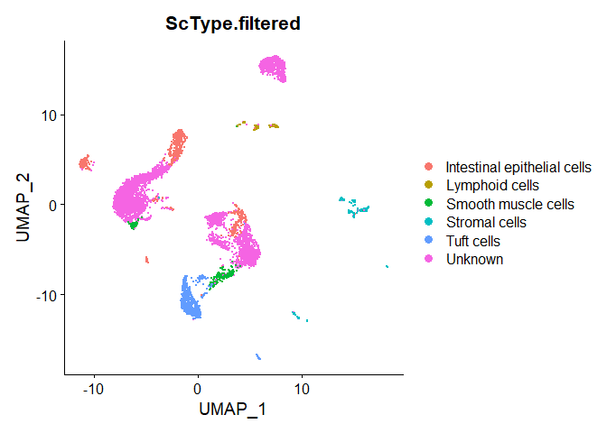
The ScType developer suggests that assignments with a score less than (number of cells in cluster)/4 are low confidence and should be set to unknown:

tmp <- data.frame(cell = colnames(experiment.merged), finalcluster = experiment.merged$finalcluster)
tmp <- left_join(tmp, cL_results.top1, by = "finalcluster")
# set assignments with scores less than ncells/4 to unknown
tmp$ScType.filtered <- ifelse(tmp$scores < tmp$ncells/4, "Unknown", tmp$ScType)
experiment.merged$ScType.filtered <- tmp$ScType.filtered
DimPlot(experiment.merged, group.by = "ScType.filtered")

Get the next Rmd file

download.file("https://raw.githubusercontent.com/ucdavis-bioinformatics-training/2022-December-Single-Cell-RNA-Seq-Analysis/main/data_analysis/scRNA_Workshop-PART6.Rmd", "scRNA_Workshop-PART6.Rmd")

Session Information

sessionInfo()
R version 4.3.1 (2023-06-16 ucrt) Platform: x86_64-w64-mingw32/x64 (64-bit) Running under: Windows 10 x64 (build 19045) Matrix products: default locale: [1] LC_COLLATE=English_United States.utf8 LC_CTYPE=English_United States.utf8 LC_MONETARY=English_United States.utf8 LC_NUMERIC=C LC_TIME=English_United States.utf8 time zone: America/Los_Angeles tzcode source: internal attached base packages: [1] stats4 stats graphics grDevices utils datasets methods base other attached packages: [1] org.Hs.eg.db_3.17.0 dplyr_1.1.2 HGNChelper_0.8.1 topGO_2.52.0 SparseM_1.81 GO.db_3.17.0 AnnotationDbi_1.62.1 IRanges_2.34.0 S4Vectors_0.38.1 Biobase_2.60.0 graph_1.78.0 BiocGenerics_0.46.0 limma_3.56.2 SeuratObject_4.1.3 Seurat_4.3.0 loaded via a namespace (and not attached): [1] RColorBrewer_1.1-3 rstudioapi_0.14 jsonlite_1.8.5 magrittr_2.0.3 spatstat.utils_3.0-3 farver_2.1.1 rmarkdown_2.22 zlibbioc_1.46.0 vctrs_0.6.3 ROCR_1.0-11 memoise_2.0.1 spatstat.explore_3.2-1 RCurl_1.98-1.12 htmltools_0.5.5 sass_0.4.6 sctransform_0.3.5 parallelly_1.36.0 KernSmooth_2.23-21 [19] bslib_0.5.0 htmlwidgets_1.6.2 ica_1.0-3 plyr_1.8.8 plotly_4.10.2 zoo_1.8-12 cachem_1.0.8 igraph_1.5.0 mime_0.12 lifecycle_1.0.3 pkgconfig_2.0.3 Matrix_1.5-4.1 R6_2.5.1 fastmap_1.1.1 GenomeInfoDbData_1.2.10 fitdistrplus_1.1-11 future_1.32.0 shiny_1.7.4 [37] digest_0.6.31 colorspace_2.1-0 patchwork_1.1.2 tensor_1.5 irlba_2.3.5.1 RSQLite_2.3.1 labeling_0.4.2 progressr_0.13.0 fansi_1.0.4 spatstat.sparse_3.0-1 httr_1.4.6 polyclip_1.10-4 abind_1.4-5 compiler_4.3.1 withr_2.5.0 bit64_4.0.5 DBI_1.1.3 highr_0.10 [55] MASS_7.3-60 tools_4.3.1 lmtest_0.9-40 zip_2.3.0 httpuv_1.6.11 future.apply_1.11.0 goftest_1.2-3 glue_1.6.2 nlme_3.1-162 promises_1.2.0.1 grid_4.3.1 Rtsne_0.16 cluster_2.1.4 reshape2_1.4.4 generics_0.1.3 gtable_0.3.3 spatstat.data_3.0-1 tidyr_1.3.0 [73] data.table_1.14.8 XVector_0.40.0 sp_1.6-1 utf8_1.2.3 spatstat.geom_3.2-1 RcppAnnoy_0.0.20 ggrepel_0.9.3 RANN_2.6.1 pillar_1.9.0 stringr_1.5.0 later_1.3.1 splines_4.3.1 lattice_0.21-8 bit_4.0.5 survival_3.5-5 deldir_1.0-9 tidyselect_1.2.0 Biostrings_2.68.1 [91] miniUI_0.1.1.1 pbapply_1.7-0 knitr_1.43 gridExtra_2.3 scattermore_1.2 xfun_0.39 matrixStats_1.0.0 stringi_1.7.12 lazyeval_0.2.2 yaml_2.3.7 evaluate_0.21 codetools_0.2-19 tibble_3.2.1 cli_3.6.1 uwot_0.1.14 xtable_1.8-4 reticulate_1.30 munsell_0.5.0 [109] jquerylib_0.1.4 GenomeInfoDb_1.36.0 Rcpp_1.0.10 globals_0.16.2 spatstat.random_3.1-5 png_0.1-8 parallel_4.3.1 ellipsis_0.3.2 blob_1.2.4 ggplot2_3.4.2 bitops_1.0-7 listenv_0.9.0 viridisLite_0.4.2 scales_1.2.1 ggridges_0.5.4 openxlsx_4.2.5.2 crayon_1.5.2 leiden_0.4.3 [127] purrr_1.0.1 rlang_1.1.1 KEGGREST_1.40.0 cowplot_1.1.1