
Last Updated: June 21, 2023
Part 7: Some other considerations in single cell datasets
Part 7.1: Integrate multiple single cell samples / batch correction
More and more experiments involve a large number of samples/datasets, that may have been prepared in separate batches. Or in the case where one would like to include or integrate publically available datasets. It is important to properly integrate these datasets, and we will see the effect the integration has at the end of this documentation.
Most of the methods that were developed to integrate single cell datasets fall into two categories. The first is the “anchor” based approach. In this approach, the first step is to select a batch as the “anchor” and convert other batches to the “anchor” batch. Among this approach, there are MNN, iMAP and SCALEX. The advantage of this approach is that different batches of cells can be studied under the same experimental conditions, and the disadvantage is that it is not possible to fully combine the features of each batch because the cell types contained in each batch are unknown. The second approach is to transform all batches of data to a low-dimensional space to correct batch effects, such as implemented in Scanorama, Harmony, DESC, BBKNN, STACAS and Seurat’s integration. This second approach has the advantage of extracting biologically relevant latent features and reducing the impact of noise, but it cannot be used for differential gene expression analysis. Many of these existing methods work well when the batches of datasets have the same cell types, however, they fail when there are different cell types involved in different datasets. Very recently (early 2022), a new approach has been developed that uses connected graphs and generative adversarial networks (GAN) to achieve the goal of eliminating nonbiological noise between batches of datasets. This new method has been demonstrated to work well both in the situation where datasets have the same cell types and in the situation where datasets may have different cell types.
In this workshop, we are going to look at Seurat’s integration approach using reciprocal PCA, which is supurior to its first integration approach using canonical correlation analysis. The basic idea is to identify cross-dataset pairs cells that are in a matched biological state (“anchors”), and use them to correct technical differences between datasets. The integration method we use has been implemented in Seurat and you can find the details of the method in its publication.
Load libraries
library(Seurat)
Load the Seurat object from the provided data and split to individual samples
The provided data is raw data that has only gone through the filtering step.
download.file("https://bioshare.bioinformatics.ucdavis.edu/bioshare/download/feb28v7lew62um4/sample_filtered.RData", "sample_filtered.RData")
load(file="sample_filtered.RData")
experiment.aggregate
## An object of class Seurat
## 21005 features across 10595 samples within 1 assay
## Active assay: RNA (21005 features, 0 variable features)
experiment.split <- SplitObject(experiment.aggregate, split.by = "ident")
Normalize and find variable features for each individual sample
By default, we employ a global-scaling normalization method LogNormalize that normalizes the gene expression measurements for each cell by the total expression, multiplies this by a scale factor (10,000 by default), and then log-transforms the data.
?NormalizeData
The function FindVariableFeatures identifies the most highly variable genes (default 2000 genes) by fitting a line to the relationship of log(variance) and log(mean) using loess smoothing, uses this information to standardize the data, then calculates the variance of the standardized data. This helps avoid selecting genes that only appear variable due to their expression level.
?FindVariableFeatures
Now, let’s carry out these two processes for each sample
experiment.split <- lapply(X = experiment.split, FUN=function(x){
  x <- NormalizeData(x)
  x <- FindVariableFeatures(x, selection.method = "vst", nfeatures = 2000)
})
Select features that are repeatedly variable across samples and run PCA on each sample
features <- SelectIntegrationFeatures(object.list = experiment.split)
experiment.split <- lapply(X = experiment.split, FUN = function(x){
  x <- ScaleData(x, features = features)
  x <- RunPCA(x, features = features)
})
Idenfity integration anchors
anchors <- FindIntegrationAnchors(object.list = experiment.split, anchor.features = features, reduction = "rpca")
Perform integration
experiment.integrated <- IntegrateData(anchorset = anchors)
Question(s)
- Explore the object “experiment.integrated” to see what information is available.
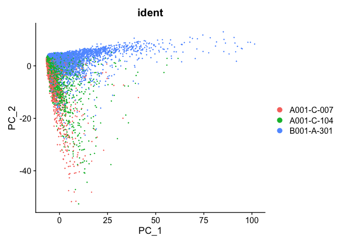
PCA plot before integration
experiment.test <- ScaleData(object=experiment.aggregate, assay="RNA")
experiment.test <- FindVariableFeatures(object=experiment.test, assay="RNA")
experiment.test <- RunPCA(object=experiment.test, assay="RNA")
DimPlot(object = experiment.test, group.by="ident", reduction="pca", shuffle=TRUE)
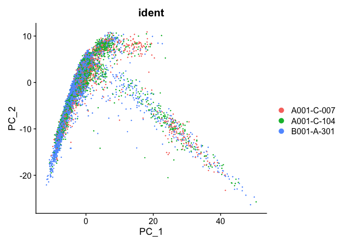
PCA plot after integration
experiment.integrated <- ScaleData(object=experiment.integrated, assay="integrated")
experiment.integrated <- RunPCA(object=experiment.integrated, assay="integrated")
DimPlot(object = experiment.integrated, group.by="ident", reduction="pca", shuffle=TRUE)
##
Save the integrated data
save(experiment.integrated, file="sample_integrated.RData")
Part 7.2: Ambient/Background RNA removal
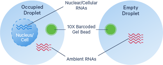
https://www.10xgenomics.com/resources/analysis-guides/introduction-to-ambient-rna-correction
Ambient RNA is a ubiquitous phenomimon for droplet-based single cell capture technologies. It captures freely floating/cell-free mRNA moleclues that are derived from ruptured, dead or dying cells, or from other source of contamination. The degree of background RNA contamination shows tissue specific characteristics, demonstrated in Madisson, et al., 2019. Single nuclei libraries also tend to produce higher background RNA, as the protocols release cytoplasmic RNA into solution, which may lead to higher background RNA in the data. Without background removal, it is still possible to get distinct cell clusters and reasonable results. The correction/removal of ambient RNA should be considered if rare and/or unknown cell types are the project goal. If the well-know major cells types are the intereste of the project, this steps is not necessary.
Approaches have been developed to address this issue, by learning the characteristics of background RNA in a dataset. There are two groups of approaches. One is to remove any cell barcode that is considered background/empty cells. This approach is what cellranger does in the preprocessing to remove all empty GEMs, which we have discussed at the step when we ran cellranger. There are other packages that can achieve the same goal, for example, EmptyNN, CellBender, DIEM, DropletQC. The other approach is to use machine learning techniques to learn the signiture of background RNA and correct each cell using the learnt feature and create a corrected gene expression profile for each barcode. In this category, there are SoupX and DecontX.
The correction of ambient RNA is a complex process and it should be considered very carefully in each study. There is no universal or fully automated process that can perform this function well for all cases and require experience and understanding of your own dataset. In addition, no approach can perform a perfect job, as in all machine learning based approaches, so choosing a library prep that reduces this issue is highly recommended if this issue is a major concern with respect to your project goal. For example, when I ran ambient RNA correction on our current dataset, there are some differences in the clustering results, however, it did not change the clustering so dramatically that cells that were clustered without this correction are now clustered with other cells instead. Here is the result
Session Information
sessionInfo()
## R version 4.2.2 (2022-10-31)
## Platform: x86_64-apple-darwin17.0 (64-bit)
## Running under: macOS Catalina 10.15.7
##
## Matrix products: default
## BLAS:   /Library/Frameworks/R.framework/Versions/4.2/Resources/lib/libRblas.0.dylib
## LAPACK: /Library/Frameworks/R.framework/Versions/4.2/Resources/lib/libRlapack.dylib
##
## locale:
## [1] en_US.UTF-8/en_US.UTF-8/en_US.UTF-8/C/en_US.UTF-8/en_US.UTF-8
##
## attached base packages:
## [1] stats     graphics  grDevices utils     datasets  methods   base
##
## other attached packages:
## [1] SeuratObject_4.1.3 Seurat_4.3.0
##
## loaded via a namespace (and not attached):
##   [1] Rtsne_0.16             colorspace_2.0-3       deldir_1.0-6
##   [4] ellipsis_0.3.2         ggridges_0.5.4         rstudioapi_0.14
##   [7] spatstat.data_3.0-0    farver_2.1.1           leiden_0.4.3
##  [10] listenv_0.8.0          ggrepel_0.9.2          fansi_1.0.3
##  [13] codetools_0.2-18       splines_4.2.2          cachem_1.0.6
##  [16] knitr_1.41             polyclip_1.10-4        jsonlite_1.8.4
##  [19] ica_1.0-3              cluster_2.1.4          png_0.1-8
##  [22] uwot_0.1.14            shiny_1.7.3            sctransform_0.3.5
##  [25] spatstat.sparse_3.0-0  compiler_4.2.2         httr_1.4.4
##  [28] assertthat_0.2.1       Matrix_1.5-3           fastmap_1.1.0
##  [31] lazyeval_0.2.2         cli_3.4.1              later_1.3.0
##  [34] htmltools_0.5.3        tools_4.2.2            igraph_1.3.5
##  [37] gtable_0.3.1           glue_1.6.2             RANN_2.6.1
##  [40] reshape2_1.4.4         dplyr_1.0.10           Rcpp_1.0.9
##  [43] scattermore_0.8        jquerylib_0.1.4        vctrs_0.5.1
##  [46] nlme_3.1-160           spatstat.explore_3.0-5 progressr_0.11.0
##  [49] lmtest_0.9-40          spatstat.random_3.0-1  xfun_0.35
##  [52] stringr_1.4.1          globals_0.16.2         mime_0.12
##  [55] miniUI_0.1.1.1         lifecycle_1.0.3        irlba_2.3.5.1
##  [58] goftest_1.2-3          future_1.29.0          MASS_7.3-58.1
##  [61] zoo_1.8-11             scales_1.2.1           promises_1.2.0.1
##  [64] spatstat.utils_3.0-1   parallel_4.2.2         RColorBrewer_1.1-3
##  [67] yaml_2.3.6             reticulate_1.28        pbapply_1.6-0
##  [70] gridExtra_2.3          ggplot2_3.4.0          sass_0.4.4
##  [73] stringi_1.7.8          highr_0.9              rlang_1.0.6
##  [76] pkgconfig_2.0.3        matrixStats_0.63.0     evaluate_0.18
##  [79] lattice_0.20-45        tensor_1.5             ROCR_1.0-11
##  [82] purrr_0.3.5            labeling_0.4.2         patchwork_1.1.2
##  [85] htmlwidgets_1.5.4      cowplot_1.1.1          tidyselect_1.2.0
##  [88] parallelly_1.32.1      RcppAnnoy_0.0.20       plyr_1.8.8
##  [91] magrittr_2.0.3         R6_2.5.1               generics_0.1.3
##  [94] DBI_1.1.3              withr_2.5.0            pillar_1.8.1
##  [97] fitdistrplus_1.1-8     survival_3.4-0         abind_1.4-5
## [100] sp_1.5-1               tibble_3.1.8           future.apply_1.10.0
## [103] KernSmooth_2.23-20     utf8_1.2.2             spatstat.geom_3.0-3
## [106] plotly_4.10.1          rmarkdown_2.18         grid_4.2.2
## [109] data.table_1.14.6      digest_0.6.30          xtable_1.8-4
## [112] tidyr_1.2.1            httpuv_1.6.6           munsell_0.5.0
## [115] viridisLite_0.4.1      bslib_0.4.1