
Introduction to box and violin plots
Box plots and their cousins, violin plots, are some of the simplest visualizations. These plots are a means of visualizing the distribution of a single continuous variable. Box and violin plots can be split to compare distributions between groups.
Box plot
The rectangular box that gives a box plot its name is drawn around the interquartile range (IQR) of the distribution, with a line marking the median, and whiskers extending to 1.5 times the IQR on either side. Outliers may be indicated with points.
Violin plot
Instead of quantile markings, violin plot has variable width designed to help the reader perceive the density of data.
Set-up
In this chapter, we will begin with the fundamentals of assembling a box plot, and then layer on additional information using graphical attributes like color and annotation text, and modify plot elements to customize figure appearance and improve readability.
Packages
We will be working extensively with ggplot2 over the course of this workshop. Part of the tidyverse ecosystem, ggplot2 is a comprehensive, flexible framework for producing highly customizable graphics of many types. We will also make use of dplyr, another tidyverse package, to clean and reshape data before plotting.
library(dplyr)
library(tidyr)
library(magrittr)
library(kableExtra)
library(ggplot2)
library(ggsignif)
library(ggExtra)
Data
We’ll use gene expression data from a single cell experiment for these plots. Typically this sort of data is stored in a complex structure which retains expression data and experiment metadata together in a single object. In this case, the data provided has been extracted from the Seurat object used in the single cell workshop. Only a small number of markers are used to limit the size of the object.
download.file("https://raw.githubusercontent.com/ucdavis-bioinformatics-training/2025-August-Intermediate-Visualization-for-Bioinformatics/refs/heads/master/R/sc_data.csv", "sc_data.csv")
sc.data <- read.csv("sc_data.csv")
Relevant metadata from the Seurat object has been added to the expression data to form a single data frame.
slice(sc.data, 1:50) %>%
  kable() %>%
  kable_styling("striped", fixed_thead = TRUE) %>%
  scroll_box(height = "200px")
| X | cell | subcluster | subcluster_ScType_filtered | SATB2 | NXPE1 | PDE3A | CFTR | HNF1A.AS1 | ADAMTSL1 | PID1 | NEO1 | XIST | NR5A2 | CNTN4 | CNTN3 | SPON1 | LEFTY1 |
|---|---|---|---|---|---|---|---|---|---|---|---|---|---|---|---|---|---|
| 1 | AAACCCAAGTTATGGA_A001-C-007 | 2 | Unknown | 2.3785758 | 2.378576 | 0.000000 | 1.774064 | 1.774064 | 0.000000 | 0.000000 | 1.7740643 | 0 | 0.000000 | 0.0000000 | 1.774064 | 0.000000 | 0 |
| 2 | AAACGCTTCTCTGCTG_A001-C-007 | 10 | Lymphoid cells | 0.0000000 | 0.000000 | 0.000000 | 2.095889 | 0.000000 | 0.000000 | 0.000000 | 0.0000000 | 0 | 0.000000 | 0.0000000 | 0.000000 | 0.000000 | 0 |
| 3 | AAAGAACGTGCTTATG_A001-C-007 | 5_1 | Intestinal epithelial cells | 2.9632015 | 3.237886 | 1.962901 | 2.583235 | 0.000000 | 1.962901 | 2.583235 | 0.0000000 | 0 | 1.962901 | 0.0000000 | 0.000000 | 0.000000 | 0 |
| 4 | AAAGAACGTTTCGCTC_A001-C-007 | 3 | Unknown | 0.0000000 | 0.000000 | 0.000000 | 0.000000 | 0.000000 | 0.000000 | 0.000000 | 0.0000000 | 0 | 0.000000 | 0.0000000 | 0.000000 | 0.000000 | 0 |
| 5 | AAAGAACTCTGGCTGG_A001-C-007 | 8 | Stromal cells | 0.0000000 | 0.000000 | 0.000000 | 0.000000 | 0.000000 | 0.000000 | 0.000000 | 0.0000000 | 0 | 0.000000 | 0.0000000 | 0.000000 | 0.000000 | 0 |
| 6 | AAAGGATTCATTACCT_A001-C-007 | 3 | Unknown | 0.0000000 | 0.000000 | 0.000000 | 0.000000 | 0.000000 | 0.000000 | 0.000000 | 0.0000000 | 0 | 0.000000 | 0.0000000 | 0.000000 | 0.000000 | 0 |
| 7 | AAAGTGACACGCTTAA_A001-C-007 | 5_2 | Unknown | 2.1190618 | 3.410926 | 2.119062 | 2.750257 | 3.134188 | 1.539372 | 0.000000 | 1.5393721 | 0 | 2.483655 | 0.0000000 | 0.000000 | 0.000000 | 0 |
| 8 | AACAAAGAGGCTAAAT_A001-C-007 | 8 | Stromal cells | 0.0000000 | 0.000000 | 1.977239 | 0.000000 | 0.000000 | 0.000000 | 0.000000 | 0.0000000 | 0 | 0.000000 | 0.0000000 | 0.000000 | 0.000000 | 0 |
| 9 | AACAAAGTCTTGGTCC_A001-C-007 | 3 | Unknown | 0.0000000 | 0.000000 | 0.000000 | 0.000000 | 1.597388 | 0.000000 | 0.000000 | 0.0000000 | 0 | 0.000000 | 0.0000000 | 0.000000 | 0.000000 | 0 |
| 10 | AACAAGACATAGAGGC_A001-C-007 | 3 | Unknown | 0.0000000 | 0.000000 | 0.000000 | 0.000000 | 0.000000 | 0.000000 | 0.000000 | 0.0000000 | 0 | 0.000000 | 0.0000000 | 0.000000 | 0.000000 | 0 |
| 11 | AACAAGAGTTTAGACC_A001-C-007 | 3 | Unknown | 0.0000000 | 0.000000 | 0.000000 | 3.102408 | 2.549943 | 0.000000 | 0.000000 | 1.7444145 | 0 | 0.000000 | 0.0000000 | 0.000000 | 0.000000 | 0 |
| 12 | AACAGGGCAATAGGAT_A001-C-007 | 3 | Unknown | 0.0000000 | 0.000000 | 0.000000 | 1.757593 | 0.000000 | 0.000000 | 0.000000 | 0.0000000 | 0 | 0.000000 | 0.0000000 | 0.000000 | 0.000000 | 0 |
| 13 | AACAGGGCATCTGTTT_A001-C-007 | 3 | Unknown | 0.0000000 | 0.000000 | 0.000000 | 2.139890 | 1.704584 | 0.000000 | 0.000000 | 0.0000000 | 0 | 0.000000 | 0.0000000 | 0.000000 | 0.000000 | 0 |
| 14 | AACAGGGGTCCCTGAG_A001-C-007 | 10 | Lymphoid cells | 0.0000000 | 0.000000 | 0.000000 | 0.000000 | 0.000000 | 0.000000 | 0.000000 | 0.0000000 | 0 | 0.000000 | 0.0000000 | 0.000000 | 0.000000 | 0 |
| 15 | AACAGGGGTGTTACAC_A001-C-007 | 3 | Unknown | 0.0000000 | 0.000000 | 0.000000 | 0.000000 | 0.000000 | 0.000000 | 0.000000 | 0.0000000 | 0 | 0.000000 | 0.0000000 | 0.000000 | 0.000000 | 0 |
| 16 | AACCAACCATGGGCAA_A001-C-007 | 3 | Unknown | 0.0000000 | 0.000000 | 0.000000 | 0.000000 | 1.393386 | 0.000000 | 0.000000 | 1.3933861 | 0 | 1.393386 | 0.0000000 | 0.000000 | 0.000000 | 0 |
| 17 | AACCACAGTCAACCAT_A001-C-007 | 3 | Unknown | 1.2432030 | 0.000000 | 0.000000 | 2.385712 | 0.000000 | 0.000000 | 0.000000 | 0.0000000 | 0 | 0.000000 | 1.2432030 | 0.000000 | 1.243203 | 0 |
| 18 | AACCATGGTACGATTC_A001-C-007 | 3 | Unknown | 0.0000000 | 0.000000 | 0.000000 | 2.493104 | 0.000000 | 0.000000 | 0.000000 | 0.0000000 | 0 | 0.000000 | 0.0000000 | 0.000000 | 0.000000 | 0 |
| 19 | AACCCAACACAGCATT_A001-C-007 | 3 | Unknown | 0.0000000 | 0.000000 | 1.046648 | 2.326344 | 1.046648 | 1.046648 | 0.000000 | 0.0000000 | 0 | 0.000000 | 0.0000000 | 0.000000 | 0.000000 | 0 |
| 20 | AACCCAAGTCGGTGTC_A001-C-007 | 2 | Unknown | 3.3415469 | 0.000000 | 1.864477 | 2.476969 | 1.864477 | 2.476969 | 2.476969 | 2.4769690 | 0 | 1.864477 | 0.0000000 | 1.864477 | 0.000000 | 0 |
| 21 | AACCTGAAGATTCGAA_A001-C-007 | 3 | Unknown | 0.0000000 | 0.000000 | 0.000000 | 0.000000 | 1.824147 | 0.000000 | 0.000000 | 0.0000000 | 0 | 0.000000 | 0.0000000 | 0.000000 | 0.000000 | 0 |
| 22 | AACCTGACAGTCAGCC_A001-C-007 | 7 | Unknown | 0.0000000 | 0.000000 | 0.000000 | 1.804794 | 0.000000 | 1.263946 | 2.787241 | 0.0000000 | 0 | 0.000000 | 0.0000000 | 0.000000 | 0.000000 | 0 |
| 23 | AACCTGAGTTGGTAGG_A001-C-007 | 7 | Unknown | 2.1502789 | 2.150279 | 2.150279 | 0.000000 | 2.783436 | 0.000000 | 2.150279 | 0.0000000 | 0 | 0.000000 | 0.0000000 | 0.000000 | 0.000000 | 0 |
| 24 | AACCTTTTCGCTCATC_A001-C-007 | 5_2 | Unknown | 0.0000000 | 0.000000 | 0.000000 | 3.062800 | 2.415349 | 0.000000 | 2.415349 | 0.0000000 | 0 | 0.000000 | 0.0000000 | 0.000000 | 0.000000 | 0 |
| 25 | AACGAAAGTATGTCTG_A001-C-007 | 5_1 | Intestinal epithelial cells | 0.0000000 | 0.000000 | 0.000000 | 0.000000 | 0.000000 | 0.000000 | 0.000000 | 0.0000000 | 0 | 0.000000 | 0.0000000 | 0.000000 | 0.000000 | 0 |
| 26 | AACGGGAAGAGGGTGG_A001-C-007 | 3 | Unknown | 0.0000000 | 0.000000 | 0.000000 | 3.790055 | 0.000000 | 0.000000 | 0.000000 | 0.0000000 | 0 | 0.000000 | 0.0000000 | 0.000000 | 0.000000 | 0 |
| 27 | AAGACAACAACACGTT_A001-C-007 | 3 | Unknown | 0.0000000 | 0.000000 | 0.000000 | 2.281880 | 0.000000 | 0.000000 | 0.000000 | 0.0000000 | 0 | 0.000000 | 0.0000000 | 0.000000 | 0.000000 | 0 |
| 28 | AAGACTCCAGCTACAT_A001-C-007 | 5_2 | Unknown | 2.1104110 | 2.741051 | 3.124780 | 2.110411 | 0.000000 | 0.000000 | 2.110411 | 0.0000000 | 0 | 2.110411 | 0.0000000 | 0.000000 | 0.000000 | 0 |
| 29 | AAGATAGCATTGGGAG_A001-C-007 | 3 | Unknown | 2.0403681 | 0.000000 | 0.000000 | 2.666317 | 0.000000 | 0.000000 | 0.000000 | 0.0000000 | 0 | 0.000000 | 0.0000000 | 0.000000 | 0.000000 | 0 |
| 30 | AAGCATCCATCCCACT_A001-C-007 | 10 | Lymphoid cells | 0.0000000 | 0.000000 | 0.000000 | 0.000000 | 0.000000 | 0.000000 | 0.000000 | 0.0000000 | 0 | 0.000000 | 0.0000000 | 0.000000 | 0.000000 | 0 |
| 31 | AAGCCATCAAGACCTT_A001-C-007 | 1 | Tuft cells | 3.5285955 | 0.000000 | 0.000000 | 0.000000 | 0.000000 | 0.000000 | 0.000000 | 0.0000000 | 0 | 0.000000 | 0.0000000 | 0.000000 | 0.000000 | 0 |
| 32 | AAGCGAGCACGAGAAC_A001-C-007 | 10 | Lymphoid cells | 2.1929693 | 0.000000 | 0.000000 | 0.000000 | 2.192969 | 0.000000 | 2.192969 | 2.1929693 | 0 | 0.000000 | 0.0000000 | 0.000000 | 0.000000 | 0 |
| 33 | AAGCGTTCAGCCTATA_A001-C-007 | 10 | Lymphoid cells | 0.0000000 | 0.000000 | 0.000000 | 0.000000 | 0.000000 | 0.000000 | 0.000000 | 0.0000000 | 0 | 0.000000 | 0.0000000 | 0.000000 | 0.000000 | 0 |
| 34 | AAGGAATAGACTCCGC_A001-C-007 | 3 | Unknown | 0.0000000 | 0.000000 | 0.000000 | 2.313001 | 2.313001 | 0.000000 | 0.000000 | 0.0000000 | 0 | 0.000000 | 0.0000000 | 0.000000 | 0.000000 | 0 |
| 35 | AAGGAATTCGTTCATT_A001-C-007 | 3 | Unknown | 0.0000000 | 0.000000 | 0.000000 | 0.000000 | 0.000000 | 0.000000 | 0.000000 | 0.0000000 | 0 | 0.000000 | 0.0000000 | 0.000000 | 0.000000 | 0 |
| 36 | AAGTACCTCGCCACTT_A001-C-007 | 3 | Unknown | 0.0000000 | 0.000000 | 0.000000 | 1.696049 | 0.000000 | 0.000000 | 0.000000 | 0.0000000 | 0 | 0.000000 | 0.0000000 | 0.000000 | 0.000000 | 0 |
| 37 | AAGTCGTGTCGCAGTC_A001-C-007 | 3 | Unknown | 0.0000000 | 0.000000 | 0.000000 | 2.988510 | 0.000000 | 0.000000 | 0.000000 | 0.0000000 | 0 | 0.000000 | 0.0000000 | 0.000000 | 0.000000 | 0 |
| 38 | AAGTCGTGTGCGAACA_A001-C-007 | 3 | Unknown | 1.5595277 | 0.000000 | 0.000000 | 0.000000 | 0.000000 | 0.000000 | 0.000000 | 1.5595277 | 0 | 0.000000 | 0.0000000 | 0.000000 | 0.000000 | 0 |
| 39 | AAGTTCGAGAACTGAT_A001-C-007 | 3 | Unknown | 0.0000000 | 0.000000 | 0.000000 | 2.275586 | 0.000000 | 2.275586 | 0.000000 | 0.0000000 | 0 | 0.000000 | 0.0000000 | 0.000000 | 0.000000 | 0 |
| 40 | AAGTTCGCAGAAGTTA_A001-C-007 | 3 | Unknown | 0.0000000 | 0.000000 | 0.000000 | 0.000000 | 0.000000 | 0.000000 | 0.000000 | 0.0000000 | 0 | 0.000000 | 0.0000000 | 0.000000 | 0.000000 | 0 |
| 41 | AAGTTCGGTACCTATG_A001-C-007 | 1 | Tuft cells | 0.0000000 | 0.000000 | 0.000000 | 2.028808 | 0.000000 | 2.028808 | 0.000000 | 0.0000000 | 0 | 0.000000 | 0.0000000 | 0.000000 | 0.000000 | 0 |
| 42 | AAGTTCGTCCTCCACA_A001-C-007 | 3 | Unknown | 0.9567933 | 0.000000 | 0.000000 | 1.759581 | 2.199076 | 0.000000 | 0.000000 | 0.9567933 | 0 | 0.000000 | 0.9567933 | 0.000000 | 0.000000 | 0 |
| 43 | AATAGAGTCGCGTGCA_A001-C-007 | 3 | Unknown | 0.0000000 | 0.000000 | 0.000000 | 0.000000 | 1.774878 | 0.000000 | 0.000000 | 0.0000000 | 0 | 0.000000 | 0.0000000 | 0.000000 | 0.000000 | 0 |
| 44 | AATCACGCAGCAATTC_A001-C-007 | 7 | Unknown | 2.0890380 | 2.089038 | 0.000000 | 2.718283 | 2.089038 | 2.089038 | 0.000000 | 0.0000000 | 0 | 0.000000 | 0.0000000 | 0.000000 | 0.000000 | 0 |
| 45 | AATGAAGCAGCCTATA_A001-C-007 | 2 | Unknown | 0.0000000 | 2.144268 | 0.000000 | 2.144268 | 3.161560 | 0.000000 | 0.000000 | 0.0000000 | 0 | 0.000000 | 0.0000000 | 0.000000 | 0.000000 | 0 |
| 46 | AATGAAGTCAGCGTCG_A001-C-007 | 1 | Tuft cells | 1.9365404 | 2.554855 | 0.000000 | 1.936540 | 2.554855 | 0.000000 | 0.000000 | 0.0000000 | 0 | 0.000000 | 0.0000000 | 0.000000 | 0.000000 | 0 |
| 47 | AATGACCCAAGCGATG_A001-C-007 | 3 | Unknown | 0.0000000 | 0.000000 | 0.000000 | 2.835224 | 1.847625 | 0.000000 | 0.000000 | 0.0000000 | 0 | 1.847625 | 0.0000000 | 0.000000 | 0.000000 | 0 |
| 48 | AATGACCTCGTAGCCG_A001-C-007 | 3 | Unknown | 0.0000000 | 0.000000 | 0.000000 | 2.407496 | 0.000000 | 0.000000 | 0.000000 | 0.0000000 | 0 | 0.000000 | 0.0000000 | 0.000000 | 0.000000 | 0 |
| 49 | AATGCCACAGGTGACA_A001-C-007 | 3 | Unknown | 0.0000000 | 1.661657 | 0.000000 | 0.000000 | 0.000000 | 0.000000 | 0.000000 | 0.0000000 | 0 | 1.661657 | 0.0000000 | 0.000000 | 0.000000 | 0 |
| 50 | AATGGAACAAGGGCAT_A001-C-007 | 7 | Unknown | 0.0000000 | 2.163120 | 0.000000 | 2.797065 | 2.163120 | 2.163120 | 0.000000 | 0.0000000 | 0 | 0.000000 | 0.0000000 | 2.797065 | 0.000000 | 0 |
Basic plot
A ggplot2 object is built in layers, with each layer inheriting
parameters from the previous elements. The parent plot is created by the
ggplot() call, and subsequent layers are added with “geoms.” Here, we
have applied geom_boxplot(), which creates box plots.
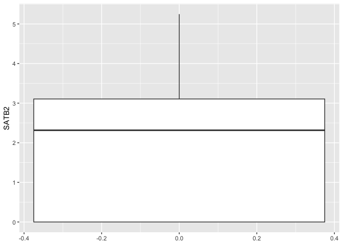
The code below generates the most basic possible box plot with our data: distribution of normalized expression values for a single gene across all cells sampled.
ggplot(data = sc.data, mapping = aes(y = SATB2)) +
  geom_boxplot()
The box plot geom accepts a number of arguments that allow you to tune its appearance. Take a look at the help statement to get an idea of the options.
?geom_boxplot
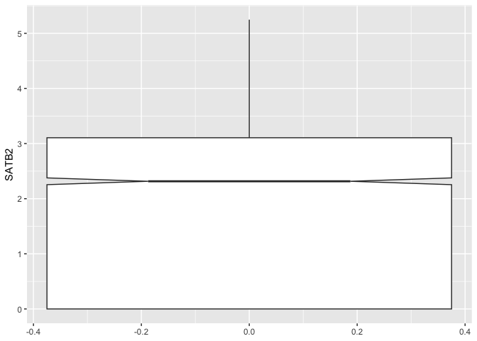
The “notch” argument controls whether a notch will be drawn at the median. Two boxes with non-overlapping notches likely represent distributions with differing medians.
ggplot(data = sc.data, mapping = aes(y = SATB2)) +
  geom_boxplot(notch = TRUE)
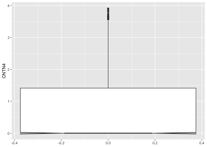
The “outlier” arguments control the appearance of any points plotted outside of the box and whiskers.
ggplot(data = sc.data, mapping = aes(y = CNTN4)) +
  geom_boxplot(notch = TRUE,
               outliers = TRUE)
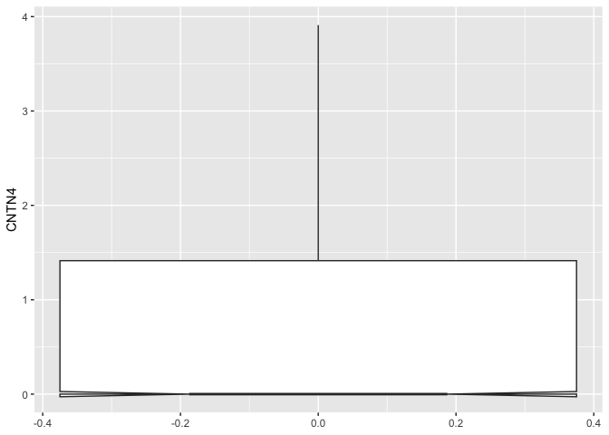
The computations underlying the box plot visualization are performed by
stat_boxplot(). By default, the length of the whiskers is 1.5 times
the interquartile range.
ggplot(data = sc.data, mapping = aes(y = CNTN4)) +
  geom_boxplot(notch = TRUE,
               coef = 2)
Comparing distributions
Our basic box plot is not as informative (or decorative) as it could be. Let’s add information from the metadata.
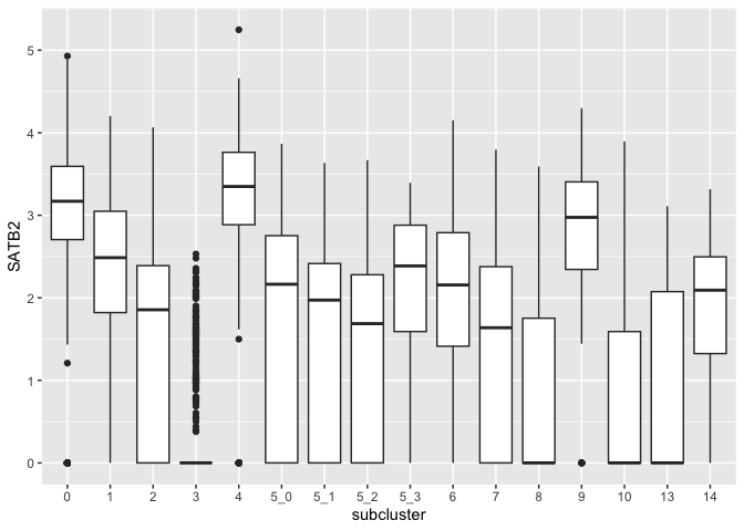
These cells have been grouped into clusters. The box plot can be split across the groups, allowing us to compare the distribution of expression values within each cell population.
Providing a categorical variable to the x axis produces a series of box plots corresponding to the levels of the variable.
ggplot(data = sc.data, mapping = aes(x = subcluster, y = SATB2)) +
  geom_boxplot()
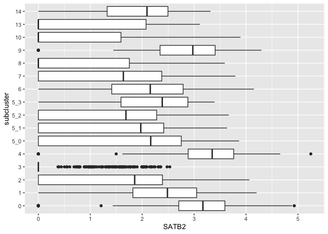
Horizontal box plots
Sometimes it may be advantageous to flip the coordinate system on its
side so that the distribution stretches from left to right instead of
vertically. This is accomplished with coord_flip().
ggplot(data = sc.data, mapping = aes(x = subcluster, y = SATB2)) +
  geom_boxplot() +
  coord_flip()
Communicate additional information using graphical attributes
While the coordinate space of a box plot communicates the values of up to two variables (one continuous and the optional second categorical), other visual qualities (aesthetics in ggplot) can be used to encode additional information, both categorical and continuous.
Box plots have the following mappable aesthetics:
- fill
- alpha
- color
- shape
- size
- linetype
- linewidth
You can assign variables to any number of these aesthetics. Some caveats apply.
Shape, and size apply to the outlier points. Shape is only suitable for categorical values, and cannot be used on very densely plotted points, where distinguishing shape becomes difficult. Meanwhile, size should be used with caution, as it implicitly communicates a sense of quantitative difference that is not appropriate for some qualitative measures (e.g. case vs control).
Color, linetype, and linewidth apply to the whiskers and box outlines. Line-based attributes can be difficult to distinguish on box plots, the interpretation of which relies heavily on the area of the boxes.
Alpha, which controls opacity, and fill apply to the box area. While alpha can be a difficult scale in which to visualize fine gradations of a continuous variable, fill is the most-used aesthetic for box and violin plots.
Fill and stroke are only useful with a subset of available point shapes; explore this documentation to understand why.
Color fill by x-axis category
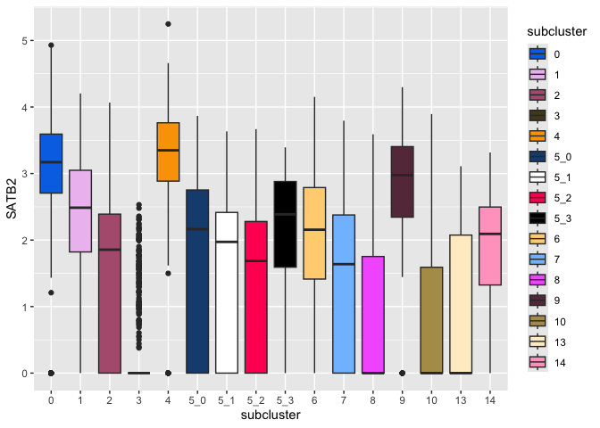
You will often see filled box plots with fill colored using the same variable as is used for the x axis. This can be useful across multi-panel visualizations to tie together the same samples visualized on different axes (e.g. a dimensionality reduction biplot and a box plot may share a color scheme to aid comprehension).
ggplot(data = sc.data, mapping = aes(x = subcluster, y = SATB2, fill = subcluster)) +
  geom_boxplot()
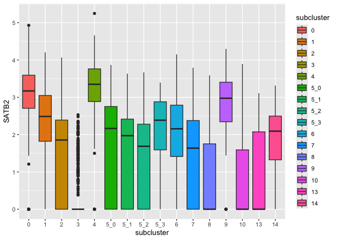
The default colors are notoriously difficult to distinguish for colorblind users. Many libraries offer palettes to extend the default color options, or you can set palettes manually.
Now that we have code for a working box plot, we can store our plot object and add to it as we go.
p <- ggplot(data = sc.data, mapping = aes(x = subcluster, y = SATB2, fill = subcluster)) + geom_boxplot()
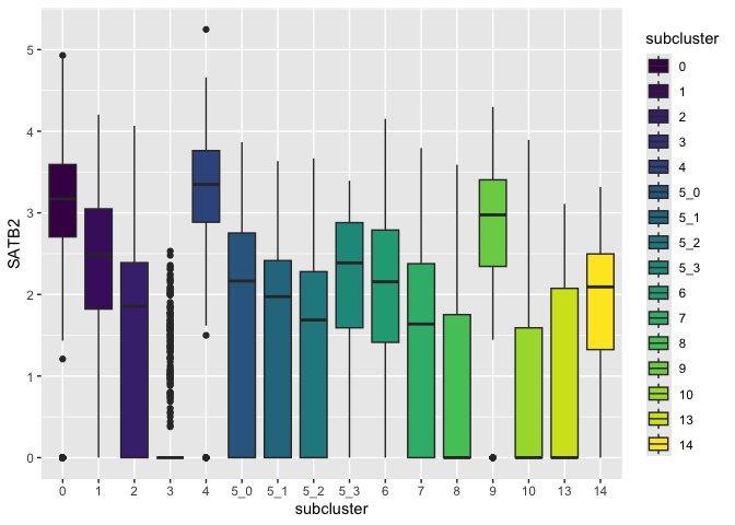
Built-in palettes: viridis
Viridis
is one of many color palette resources. To access the viridis palettes
seamlessly within ggplot2, we can call the scale_fill_viridis_ family
of functions: d for discrete data, b for binned data, and c for
continuous data.
p + scale_fill_viridis_d()
Custom color palettes
The simplest way to set custom colors for a ggplot object is with
scale_fill_manual(). These colors are based on a selection of web
accessible colors generated by
palette.es.
While the 5 color version generated by the site is relatively
accessible, this expanded color palette is not.
custom.palette <- c("#0074e6", "#eec1f1", "#b35e7e", "#534623", "#faa300",
                    "#194d80", "white", "#ff0062", "black", "#ffd380",
                    "#80c0ff", "#f566ff", "#663648", "#b39b59", "#ffedcc",
                    "#ffa6c8")
p + scale_fill_manual(values = custom.palette)
Color fill independent of x-axis
When no value is supplied to x, the fill will be used to split the box plot.
ggplot(data = sc.data, mapping = aes(y = SATB2, fill = subcluster_ScType_filtered)) +
  geom_boxplot() +
  scale_fill_viridis_d(option = "turbo", name = "Putative cell type") +
  theme(axis.text.x = element_text(angle = 45, hjust = 1))
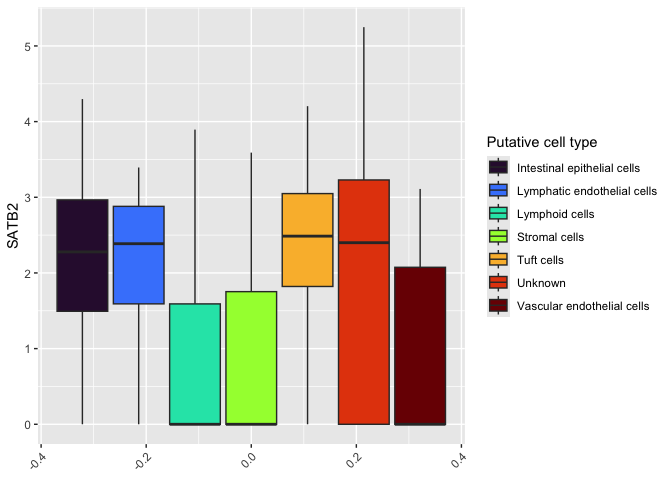
Coloring by putative cell reveals that cell type assignment was inconclusive for a large number of cells. Locating this box toward the center of our plot, and filling it with a bright color distracts from the differences in expression we observe between cells that were successfully assigned.
To do this, we convert the character vector “subcluster_ScType_filtered” in our data frame to a factor, and set the levels to control the ordering.
sc.data$putative <- factor(gsub("Unknown", NA, sc.data$subcluster_ScType_filtered),
                           levels = c("Vascular endothelial cells",
                                      "Lymphoid cells",
                                      "Stromal cells",
                                      "Tuft cells",
                                      "Lymphatic endothelial cells",
                                      "Intestinal epithelial cells"))
ggplot(data = sc.data, mapping = aes(y = SATB2, fill = putative)) +
  geom_boxplot() +
  scale_fill_viridis_d(option = "turbo",
                       name = "Putative cell type",
                       begin = 0.1,
                       end = 0.9,
                       na.value = "gray90")
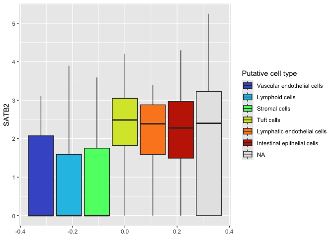
The fill scale function also offers the option of setting a shade for
missing data. Here we have selected a low-contrast light gray color.
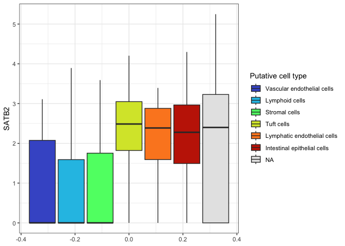
With this gray color used for NA, a white background may be preferable.
All graphical elements of a ggplot object are modifiable, and a number
of pre-built themes exist. The default theme is theme_gray().
ggplot(data = sc.data, mapping = aes(y = SATB2, fill = putative)) +
  geom_boxplot() +
  scale_fill_viridis_d(option = "turbo",
                       name = "Putative cell type",
                       begin = 0.1,
                       end = 0.9,
                       na.value = "gray90") +
  theme_bw()
Reshaping data for improved visualizations
If more than one marker is of interest, we can display these on a shared set of axes by reshaping the data frame to put the expression values in the same column. Associated gene symbols are moved to another column, making the data frame much longer and narrower.
pivot_longer(sc.data, cols = SATB2:LEFTY1, names_to = "gene", values_to = "normalized.counts") %>%
  slice(1:50) %>%
  kable() %>%
  kable_styling("striped", fixed_thead = TRUE) %>%
  scroll_box(height = "200px")
| X | cell | subcluster | subcluster_ScType_filtered | putative | gene | normalized.counts |
|---|---|---|---|---|---|---|
| 1 | AAACCCAAGTTATGGA_A001-C-007 | 2 | Unknown | NA | SATB2 | 2.378576 |
| 1 | AAACCCAAGTTATGGA_A001-C-007 | 2 | Unknown | NA | NXPE1 | 2.378576 |
| 1 | AAACCCAAGTTATGGA_A001-C-007 | 2 | Unknown | NA | PDE3A | 0.000000 |
| 1 | AAACCCAAGTTATGGA_A001-C-007 | 2 | Unknown | NA | CFTR | 1.774064 |
| 1 | AAACCCAAGTTATGGA_A001-C-007 | 2 | Unknown | NA | HNF1A.AS1 | 1.774064 |
| 1 | AAACCCAAGTTATGGA_A001-C-007 | 2 | Unknown | NA | ADAMTSL1 | 0.000000 |
| 1 | AAACCCAAGTTATGGA_A001-C-007 | 2 | Unknown | NA | PID1 | 0.000000 |
| 1 | AAACCCAAGTTATGGA_A001-C-007 | 2 | Unknown | NA | NEO1 | 1.774064 |
| 1 | AAACCCAAGTTATGGA_A001-C-007 | 2 | Unknown | NA | XIST | 0.000000 |
| 1 | AAACCCAAGTTATGGA_A001-C-007 | 2 | Unknown | NA | NR5A2 | 0.000000 |
| 1 | AAACCCAAGTTATGGA_A001-C-007 | 2 | Unknown | NA | CNTN4 | 0.000000 |
| 1 | AAACCCAAGTTATGGA_A001-C-007 | 2 | Unknown | NA | CNTN3 | 1.774064 |
| 1 | AAACCCAAGTTATGGA_A001-C-007 | 2 | Unknown | NA | SPON1 | 0.000000 |
| 1 | AAACCCAAGTTATGGA_A001-C-007 | 2 | Unknown | NA | LEFTY1 | 0.000000 |
| 2 | AAACGCTTCTCTGCTG_A001-C-007 | 10 | Lymphoid cells | Lymphoid cells | SATB2 | 0.000000 |
| 2 | AAACGCTTCTCTGCTG_A001-C-007 | 10 | Lymphoid cells | Lymphoid cells | NXPE1 | 0.000000 |
| 2 | AAACGCTTCTCTGCTG_A001-C-007 | 10 | Lymphoid cells | Lymphoid cells | PDE3A | 0.000000 |
| 2 | AAACGCTTCTCTGCTG_A001-C-007 | 10 | Lymphoid cells | Lymphoid cells | CFTR | 2.095889 |
| 2 | AAACGCTTCTCTGCTG_A001-C-007 | 10 | Lymphoid cells | Lymphoid cells | HNF1A.AS1 | 0.000000 |
| 2 | AAACGCTTCTCTGCTG_A001-C-007 | 10 | Lymphoid cells | Lymphoid cells | ADAMTSL1 | 0.000000 |
| 2 | AAACGCTTCTCTGCTG_A001-C-007 | 10 | Lymphoid cells | Lymphoid cells | PID1 | 0.000000 |
| 2 | AAACGCTTCTCTGCTG_A001-C-007 | 10 | Lymphoid cells | Lymphoid cells | NEO1 | 0.000000 |
| 2 | AAACGCTTCTCTGCTG_A001-C-007 | 10 | Lymphoid cells | Lymphoid cells | XIST | 0.000000 |
| 2 | AAACGCTTCTCTGCTG_A001-C-007 | 10 | Lymphoid cells | Lymphoid cells | NR5A2 | 0.000000 |
| 2 | AAACGCTTCTCTGCTG_A001-C-007 | 10 | Lymphoid cells | Lymphoid cells | CNTN4 | 0.000000 |
| 2 | AAACGCTTCTCTGCTG_A001-C-007 | 10 | Lymphoid cells | Lymphoid cells | CNTN3 | 0.000000 |
| 2 | AAACGCTTCTCTGCTG_A001-C-007 | 10 | Lymphoid cells | Lymphoid cells | SPON1 | 0.000000 |
| 2 | AAACGCTTCTCTGCTG_A001-C-007 | 10 | Lymphoid cells | Lymphoid cells | LEFTY1 | 0.000000 |
| 3 | AAAGAACGTGCTTATG_A001-C-007 | 5_1 | Intestinal epithelial cells | Intestinal epithelial cells | SATB2 | 2.963201 |
| 3 | AAAGAACGTGCTTATG_A001-C-007 | 5_1 | Intestinal epithelial cells | Intestinal epithelial cells | NXPE1 | 3.237886 |
| 3 | AAAGAACGTGCTTATG_A001-C-007 | 5_1 | Intestinal epithelial cells | Intestinal epithelial cells | PDE3A | 1.962901 |
| 3 | AAAGAACGTGCTTATG_A001-C-007 | 5_1 | Intestinal epithelial cells | Intestinal epithelial cells | CFTR | 2.583235 |
| 3 | AAAGAACGTGCTTATG_A001-C-007 | 5_1 | Intestinal epithelial cells | Intestinal epithelial cells | HNF1A.AS1 | 0.000000 |
| 3 | AAAGAACGTGCTTATG_A001-C-007 | 5_1 | Intestinal epithelial cells | Intestinal epithelial cells | ADAMTSL1 | 1.962901 |
| 3 | AAAGAACGTGCTTATG_A001-C-007 | 5_1 | Intestinal epithelial cells | Intestinal epithelial cells | PID1 | 2.583235 |
| 3 | AAAGAACGTGCTTATG_A001-C-007 | 5_1 | Intestinal epithelial cells | Intestinal epithelial cells | NEO1 | 0.000000 |
| 3 | AAAGAACGTGCTTATG_A001-C-007 | 5_1 | Intestinal epithelial cells | Intestinal epithelial cells | XIST | 0.000000 |
| 3 | AAAGAACGTGCTTATG_A001-C-007 | 5_1 | Intestinal epithelial cells | Intestinal epithelial cells | NR5A2 | 1.962901 |
| 3 | AAAGAACGTGCTTATG_A001-C-007 | 5_1 | Intestinal epithelial cells | Intestinal epithelial cells | CNTN4 | 0.000000 |
| 3 | AAAGAACGTGCTTATG_A001-C-007 | 5_1 | Intestinal epithelial cells | Intestinal epithelial cells | CNTN3 | 0.000000 |
| 3 | AAAGAACGTGCTTATG_A001-C-007 | 5_1 | Intestinal epithelial cells | Intestinal epithelial cells | SPON1 | 0.000000 |
| 3 | AAAGAACGTGCTTATG_A001-C-007 | 5_1 | Intestinal epithelial cells | Intestinal epithelial cells | LEFTY1 | 0.000000 |
| 4 | AAAGAACGTTTCGCTC_A001-C-007 | 3 | Unknown | NA | SATB2 | 0.000000 |
| 4 | AAAGAACGTTTCGCTC_A001-C-007 | 3 | Unknown | NA | NXPE1 | 0.000000 |
| 4 | AAAGAACGTTTCGCTC_A001-C-007 | 3 | Unknown | NA | PDE3A | 0.000000 |
| 4 | AAAGAACGTTTCGCTC_A001-C-007 | 3 | Unknown | NA | CFTR | 0.000000 |
| 4 | AAAGAACGTTTCGCTC_A001-C-007 | 3 | Unknown | NA | HNF1A.AS1 | 0.000000 |
| 4 | AAAGAACGTTTCGCTC_A001-C-007 | 3 | Unknown | NA | ADAMTSL1 | 0.000000 |
| 4 | AAAGAACGTTTCGCTC_A001-C-007 | 3 | Unknown | NA | PID1 | 0.000000 |
| 4 | AAAGAACGTTTCGCTC_A001-C-007 | 3 | Unknown | NA | NEO1 | 0.000000 |
sc.pivot <- pivot_longer(sc.data, cols = SATB2:LEFTY1, names_to = "gene", values_to = "normalized.counts")
Reshaping the data frame this way allows us to use “gene” to set fill color, while the y-axis is relabled “normalized.counts.”
filter(sc.pivot, gene %in% c("PDE3A", "CFTR", "ADAMTSL1")) %>%
  ggplot(mapping = aes(x = subcluster, y = normalized.counts, fill = gene)) +
  geom_boxplot() +
  scale_fill_viridis_d() +
  theme_bw()
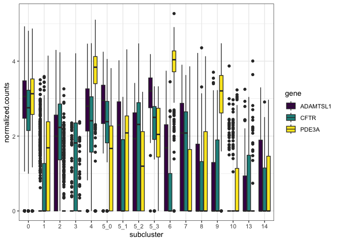
Notice that the x-axis and fill are assigned independently, resulting in three boxes plotted for each sub-cluster.
Displaying multiple categorical variables
If we want to examine the relationship between our three markers of interest from the previous figure split over each putative cell type, we can accomplish this one of three ways:
- use putative cell type as x and gene as fill
- use gene as fill and facet by putative cell type
- create a facet grid using gene ~ putative cell type
Set fill and x independently
As in the previous figure, we can simply set assign the fill and x aesthetics to different categorical values.
filter(sc.pivot, gene %in% c("PDE3A", "CFTR", "ADAMTSL1")) %>%
  ggplot(mapping = aes(x = putative, y = normalized.counts, fill = gene)) +
  geom_boxplot() +
  scale_fill_viridis_d() +
  theme_bw()
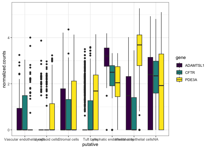
Due to the long cell type names, the x-axis is unreadable. Let’s change
the angle of the text in order to prevent overlapping. The theme()
function in ggplot2 allows access to the plot elements individually,
allowing us to fine-tune the axis text appearance (among many other
things!).
filter(sc.pivot, gene %in% c("PDE3A", "CFTR", "ADAMTSL1")) %>%
  ggplot(mapping = aes(x = putative, y = normalized.counts, fill = gene)) +
  geom_boxplot() +
  scale_fill_viridis_d() +
  theme_bw() +
  theme(axis.text.x = element_text(angle = 45, hjust = 1))
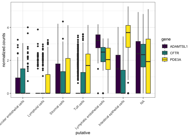
We can also suppress the unecessary plot x-axis and legend titles.
filter(sc.pivot, gene %in% c("PDE3A", "CFTR", "ADAMTSL1")) %>%
  ggplot(mapping = aes(x = putative, y = normalized.counts, fill = gene)) +
  geom_boxplot() +
  scale_fill_viridis_d() +
  theme_bw() +
  theme(axis.text.x = element_text(angle = 45, hjust = 1),
        axis.title.x = element_blank(),
        legend.title = element_blank())
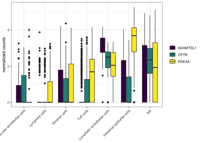
The labs() function lets us specify labels, captions and titles for
the plot.
filter(sc.pivot, gene %in% c("PDE3A", "CFTR", "ADAMTSL1")) %>%
  ggplot(mapping = aes(x = putative, y = normalized.counts, fill = gene)) +
  geom_boxplot() +
  scale_fill_viridis_d() +
  labs(y = "Normalized counts") +
  theme_bw() +
  theme(axis.text.x = element_text(angle = 45, hjust = 1),
        axis.title.x = element_blank(),
        legend.title = element_blank())

To change the axis tick labels, use scale_x_discrete().
filter(sc.pivot, gene %in% c("PDE3A", "CFTR", "ADAMTSL1")) %>%
  ggplot(mapping = aes(x = putative, y = normalized.counts, fill = gene)) +
  geom_boxplot() +
  scale_fill_viridis_d() +
  labs(y = "Normalized counts") +
  theme_bw() +
  scale_x_discrete(labels = c(levels(sc.pivot$putative), "Unassigned")) +
  theme(axis.text.x = element_text(angle = 45, hjust = 1),
        axis.title.x = element_blank(),
        legend.title = element_blank())
 ##
Facets
##
Facets
Faceting creates multiple sub-plots, which allow us to visualize more levels of categorical variation without adding additional colors.
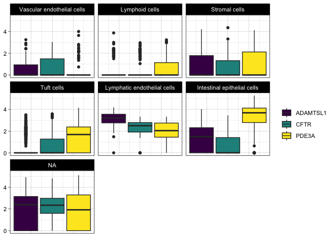
Fill by cell type and facet by gene
filter(sc.pivot, gene %in% c("PDE3A", "CFTR", "ADAMTSL1")) %>%
  ggplot(mapping = aes(y = normalized.counts, fill = putative)) +
  geom_boxplot() +
  facet_wrap(~gene) +
  scale_fill_viridis_d(option = "turbo",
                       name = "Putative cell type",
                       begin = 0.1,
                       end = 0.9,
                       na.value = "gray90") +
  theme_bw() +
  theme(legend.title = element_blank(),
        axis.text.x = element_blank(),
        axis.ticks.x = element_blank(),
        axis.title = element_blank())
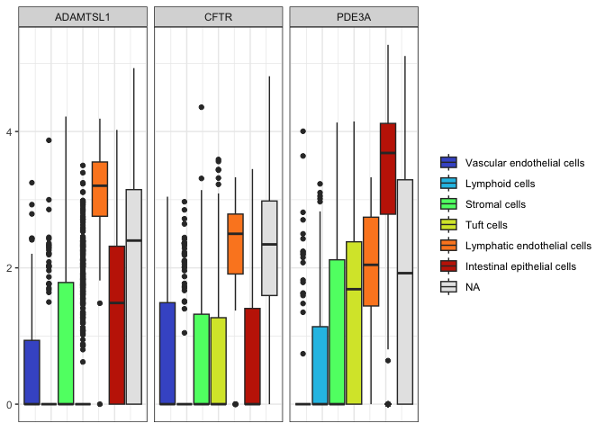
When crafting your box plot, try to make the most important comparison easy for viewers. In this case, filling by gene and faceting by cell type may be more useful.
Fill by gene and facet by cell type
filter(sc.pivot, gene %in% c("PDE3A", "CFTR", "ADAMTSL1")) %>%
  ggplot(mapping = aes(y = normalized.counts, fill = gene)) +
  geom_boxplot() +
  facet_wrap(~putative) +
  scale_fill_viridis_d() +
  theme_linedraw() +
  theme(legend.title = element_blank(),
        axis.text.x = element_blank(),
        axis.ticks.x = element_blank(),
        axis.title = element_blank())
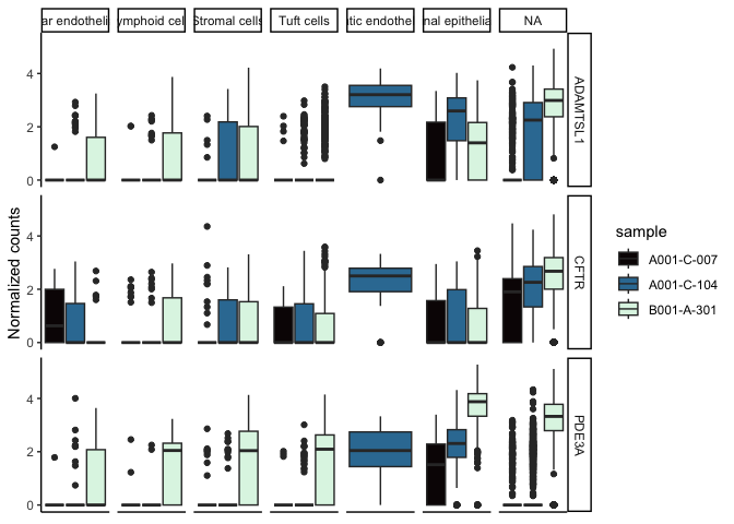
Create a gene by cell type grid
If we wanted to examine the relationship between the sample identity, cell type, and gene expression, we can create a grid that allows us to view all three simultaneously.
sc.pivot$sample <- sapply(strsplit(sc.pivot$cell, split = "_", fixed = TRUE), "[[", 2L)
filter(sc.pivot, gene %in% c("PDE3A", "CFTR", "ADAMTSL1")) %>%
  ggplot(mapping = aes(y = normalized.counts, fill = sample)) +
  geom_boxplot() +
  facet_grid(gene~putative) +
  scale_fill_viridis_d(option = "mako") +
  theme_classic() +
  theme(axis.text.x = element_blank(),
        axis.ticks.x = element_blank()) +
  labs(y = "Normalized counts")
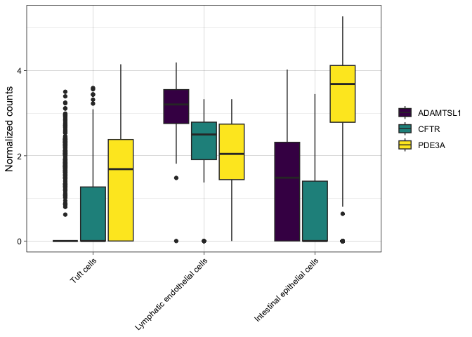
Subset the data
If some comparisons are irrelevant, you can subset the data for the sake of clarity.
filter(sc.pivot,
       gene %in% c("PDE3A", "CFTR", "ADAMTSL1"),
       putative %in% c("Intestinal epithelial cells", "Lymphatic endothelial cells", "Tuft cells")) %>%
  ggplot(mapping = aes(x = putative, y = normalized.counts, fill = gene)) +
  geom_boxplot() +
  scale_fill_viridis_d() +
  labs(y = "Normalized counts") +
  theme_linedraw() +
  theme(axis.title.x = element_blank(),
        legend.title = element_blank(),
        axis.text.x = element_text(angle = 45, hjust = 1))
Annotations
Box plots are, by their nature, fairly simple. Adding annotations to the box plot to highlight comparisons of interest or communicate additional information can make them more informative without becoming overly complex.
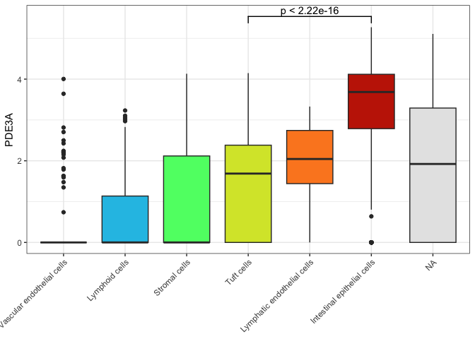
One common annotation for box plots is the significance bracket. These are visual indicators of statistically significant differences between means. They may be marked with the p-value for the test, or with asterisks.
It is possible to add significance annotations manually, but we will be using the library ggsignif.
ggplot(data = sc.data, mapping = aes(x = putative, y = PDE3A, fill = putative)) +
  geom_boxplot() +
  scale_fill_viridis_d(option = "turbo",
                       begin = 0.1,
                       end = 0.9,
                       na.value = "gray90") +
  guides(fill = "none") +
  geom_signif(comparisons = list(c("Tuft cells", "Intestinal epithelial cells"))) +
  theme_bw() +
  theme(axis.title.x = element_blank(),
        axis.text.x = element_text(angle = 45, hjust = 1))
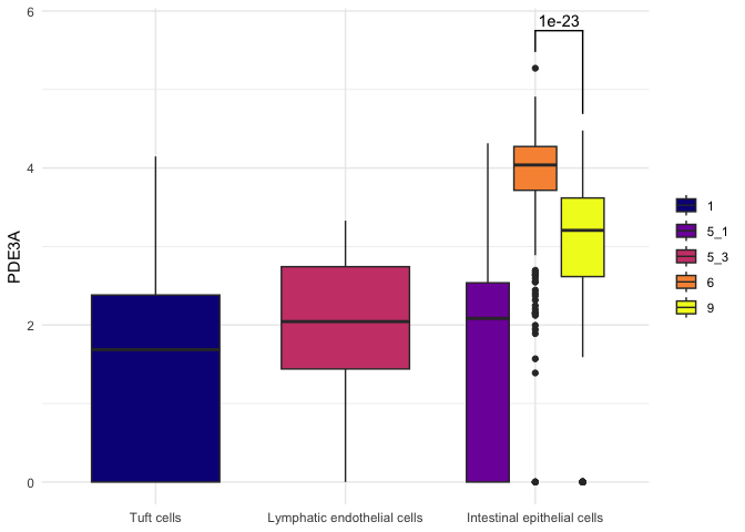
The significance test geom produced by ggsignif is compatible with coord_flip and faceting, but does require manual adjustment when categorical values on the x axis are broken up by the fill argument and position_dodge comes into play.
anno <- t.test(sc.data$PDE3A[sc.data$subcluster == "6"],
               sc.data$PDE3A[sc.data$subcluster == "9"])
filter(sc.data, putative %in% c("Tuft cells", "Lymphatic endothelial cells", "Intestinal epithelial cells")) %>%
  ggplot(mapping = (aes(x = putative, y = PDE3A, fill = subcluster))) +
  geom_boxplot() +
  geom_signif(annotation = formatC(anno$p.value, digits = 1),
              y_position = 5.75,
              xmin = 3,
              xmax = 3.25,
              tip_length = c(0.05,0.2)) +
  scale_fill_viridis_d(option = "plasma") +
  theme_minimal() +
  theme(axis.title.x = element_blank(),
        legend.title = element_blank())
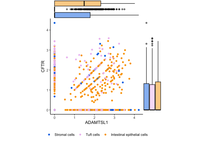
Marginal plots
Box plots can also be useful in the context of annotating other types of
plots. For example, in a densely plotted scatter plot, you may want
marginal box plots to help readers accurately perceive the distribution
of values on one or both axes. This can help you combat misleading
over-plotting. The ggMarginal() function from ggExtra provides access
to three types of marginal plots, including a box plot.
p <- filter(sc.data, putative %in% c("Intestinal epithelial cells", "Tuft cells", "Stromal cells")) %>%
  ggplot(mapping = aes(x = ADAMTSL1, y = CFTR, color = putative, fill = putative)) +
  geom_point() +
  scale_color_manual(values = custom.palette[c(1,2,5)]) +
  coord_fixed() +
  theme_classic()
ggMarginal(p + theme(legend.position = "bottom", legend.title = element_blank()), type = "boxplot", groupFill = TRUE)
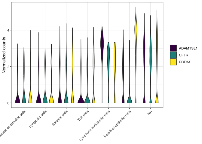
Violin plots
Violin plots are very similar to box plots. In some cases, you can
simply substitute geom_violin() in place of geom_boxplot(). However,
be aware that violin plots require a mapping for the x aesthetic.
filter(sc.pivot, gene %in% c("PDE3A", "CFTR", "ADAMTSL1")) %>%
  ggplot(mapping = aes(x = putative, y = normalized.counts, fill = gene)) +
  geom_violin() +
  scale_fill_viridis_d() +
  labs(y = "Normalized counts") +
  theme_bw() +
  theme(axis.text.x = element_text(angle = 45, hjust = 1),
        axis.title.x = element_blank(),
        legend.title = element_blank())
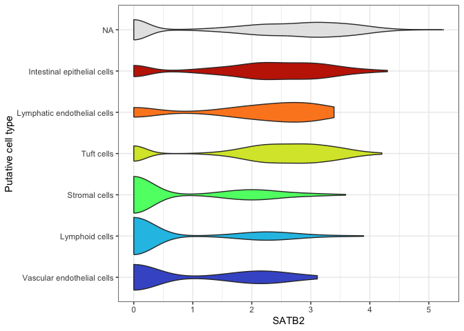
ggplot(data = sc.data, mapping = aes(x = putative, y = SATB2, fill = putative)) +
  geom_violin() +
  scale_fill_viridis_d(option = "turbo",
                       begin = 0.1,
                       end = 0.9,
                       na.value = "gray90") +
  guides(fill = "none") +
  labs(x = "Putative cell type") +
  coord_flip() +
  theme_bw()
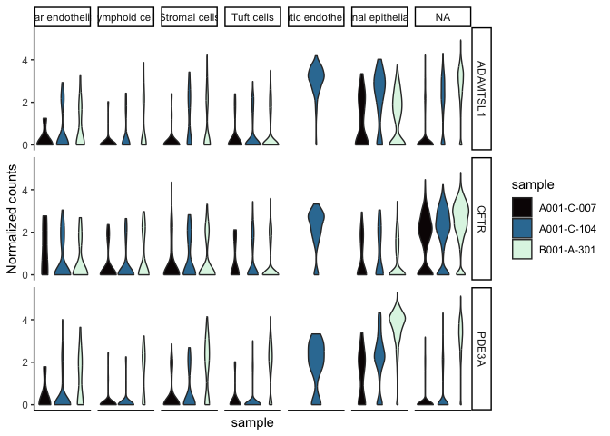
filter(sc.pivot, gene %in% c("PDE3A", "CFTR", "ADAMTSL1")) %>%
  ggplot(mapping = aes(y = normalized.counts, x = sample, fill = sample)) +
  geom_violin() +
  facet_grid(gene~putative) +
  scale_fill_viridis_d(option = "mako") +
  theme_classic() +
  theme(axis.text.x = element_blank(),
        axis.ticks.x = element_blank()) +
  labs(y = "Normalized counts")
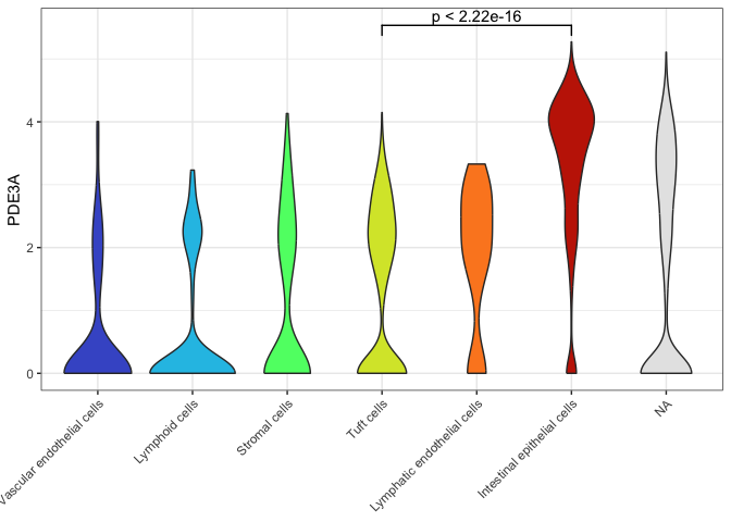
Significance brackets are not common on violin plots, but if desired, it functions the same way as on a box plot.
ggplot(data = sc.data, mapping = aes(x = putative, y = PDE3A, fill = putative)) +
  geom_violin() +
  scale_fill_viridis_d(option = "turbo",
                       begin = 0.1,
                       end = 0.9,
                       na.value = "gray90") +
  guides(fill = "none") +
  geom_signif(comparisons = list(c("Tuft cells", "Intestinal epithelial cells"))) +
  theme_bw() +
  theme(axis.title.x = element_blank(),
        axis.text.x = element_text(angle = 45, hjust = 1))
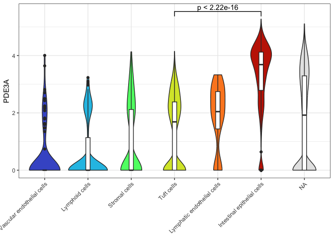
 Occasionally, you will see a box plot superimposed on the violin forms.
In this case, be sure to move the fill assignment inside the
geom_violin() call so that the box plots remain unfilled (this makes
them easier to perceive).
Occasionally, you will see a box plot superimposed on the violin forms.
In this case, be sure to move the fill assignment inside the
geom_violin() call so that the box plots remain unfilled (this makes
them easier to perceive).
ggplot(data = sc.data, mapping = aes(x = putative, y = PDE3A)) +
  geom_violin(mapping = aes(fill = putative)) +
  geom_boxplot(width = 0.1) +
  scale_fill_viridis_d(option = "turbo",
                       begin = 0.1,
                       end = 0.9,
                       na.value = "gray90") +
  guides(fill = "none") +
  geom_signif(comparisons = list(c("Tuft cells", "Intestinal epithelial cells"))) +
  theme_bw() +
  theme(axis.title.x = element_blank(),
        axis.text.x = element_text(angle = 45, hjust = 1))
Prepare for the next section
download.file("https://raw.githubusercontent.com/ucdavis-bioinformatics-training/2025-August-Intermediate-Visualization-for-Bioinformatics/refs/heads/master/R/02-scatterplot.Rmd", "02-scatterplot.Rmd")
sessionInfo()
## R version 4.5.1 (2025-06-13)
## Platform: aarch64-apple-darwin20
## Running under: macOS Monterey 12.4
##
## Matrix products: default
## BLAS:   /Library/Frameworks/R.framework/Versions/4.5-arm64/Resources/lib/libRblas.0.dylib
## LAPACK: /Library/Frameworks/R.framework/Versions/4.5-arm64/Resources/lib/libRlapack.dylib;  LAPACK version 3.12.1
##
## locale:
## [1] en_US.UTF-8/en_US.UTF-8/en_US.UTF-8/C/en_US.UTF-8/en_US.UTF-8
##
## time zone: America/Los_Angeles
## tzcode source: internal
##
## attached base packages:
## [1] stats     graphics  grDevices utils     datasets  methods   base
##
## other attached packages:
## [1] ggExtra_0.10.1   ggsignif_0.6.4   ggplot2_3.5.2    kableExtra_1.4.0
## [5] magrittr_2.0.3   tidyr_1.3.1      dplyr_1.1.4
##
## loaded via a namespace (and not attached):
##  [1] miniUI_0.1.2       gtable_0.3.6       compiler_4.5.1     promises_1.3.3
##  [5] Rcpp_1.1.0         tidyselect_1.2.1   xml2_1.3.8         stringr_1.5.1
##  [9] later_1.4.2        systemfonts_1.2.3  scales_1.4.0       textshaping_1.0.1
## [13] yaml_2.3.10        fastmap_1.2.0      mime_0.13          R6_2.6.1
## [17] labeling_0.4.3     generics_0.1.4     knitr_1.50         tibble_3.3.0
## [21] shiny_1.11.1       svglite_2.2.1      pillar_1.11.0      RColorBrewer_1.1-3
## [25] rlang_1.1.6        stringi_1.8.7      httpuv_1.6.16      xfun_0.52
## [29] viridisLite_0.4.2  cli_3.6.5          withr_3.0.2        digest_0.6.37
## [33] grid_4.5.1         xtable_1.8-4       rstudioapi_0.17.1  lifecycle_1.0.4
## [37] vctrs_0.6.5        evaluate_1.0.4     glue_1.8.0         farver_2.1.2
## [41] rmarkdown_2.29     purrr_1.1.0        tools_4.5.1        pkgconfig_2.0.3
## [45] htmltools_0.5.8.1