
Differential Gene Expression Analysis in R
- Differential Gene Expression (DGE) between conditions is determined from count data
- Generally speaking differential expression analysis is performed in a very similar manner to metabolomics, proteomics, or DNA microarrays, once normalization and transformations have been performed.
A lot of RNA-seq analysis has been done in R and so there are many packages available to analyze and view this data. Two of the most commonly used are:
- DESeq2, developed by Simon Anders (also created htseq) in Wolfgang Huber’s group at EMBL
- edgeR and Voom (extension to Limma [microarrays] for RNA-seq), developed out of Gordon Smyth’s group from the Walter and Eliza Hall Institute of Medical Research in Australia
http://bioconductor.org/packages/release/BiocViews.html#___RNASeq
Differential Expression Analysis with Limma-Voom
limma is an R package that was originally developed for differential expression (DE) analysis of gene expression microarray data.
voom is a function in the limma package that transforms RNA-Seq data for use with limma.
Together they allow fast, flexible, and powerful analyses of RNA-Seq data. Limma-voom is our tool of choice for DE analyses because it:
-
Allows for incredibly flexible model specification (you can include multiple categorical and continuous variables, allowing incorporation of almost any kind of metadata).
-
Based on simulation studies, maintains the false discovery rate at or below the nominal rate, unlike some other packages.
-
Empirical Bayes smoothing of gene-wise standard deviations provides increased power.
Basic Steps of Differential Gene Expression
- Read count data and annotation into R and preprocessing.
- Calculate normalization factors (sample-specific adjustments)
- Filter genes (uninteresting genes, e.g. unexpressed)
- Account for expression-dependent variability by transformation, weighting, or modeling
- Fitting a linear model
- Perform statistical comparisons of interest (using contrasts)
- Adjust for multiple testing, Benjamini-Hochberg (BH) or q-value
- Check results for confidence
- Attach annotation if available and write tables
1. Read in the counts table and create our DGEList
counts <- read.delim("rnaseq_workshop_counts.txt", row.names = 1)
head(counts)
##                      mouse_110_WT_C mouse_110_WT_NC mouse_148_WT_C
## ENSMUSG00000102693.2              0               0              0
## ENSMUSG00000064842.3              0               0              0
## ENSMUSG00000051951.6              0               0              0
## ENSMUSG00000102851.2              0               0              0
## ENSMUSG00000103377.2              0               0              0
## ENSMUSG00000104017.2              0               0              0
##                      mouse_148_WT_NC mouse_158_WT_C mouse_158_WT_NC
## ENSMUSG00000102693.2               0              0               0
## ENSMUSG00000064842.3               0              0               0
## ENSMUSG00000051951.6               0              0               0
## ENSMUSG00000102851.2               0              0               0
## ENSMUSG00000103377.2               0              0               0
## ENSMUSG00000104017.2               0              0               0
##                      mouse_183_KOMIR150_C mouse_183_KOMIR150_NC
## ENSMUSG00000102693.2                    0                     0
## ENSMUSG00000064842.3                    0                     0
## ENSMUSG00000051951.6                    0                     0
## ENSMUSG00000102851.2                    0                     0
## ENSMUSG00000103377.2                    0                     0
## ENSMUSG00000104017.2                    0                     0
##                      mouse_198_KOMIR150_C mouse_198_KOMIR150_NC
## ENSMUSG00000102693.2                    0                     0
## ENSMUSG00000064842.3                    0                     0
## ENSMUSG00000051951.6                    0                     0
## ENSMUSG00000102851.2                    0                     0
## ENSMUSG00000103377.2                    0                     0
## ENSMUSG00000104017.2                    0                     0
##                      mouse_206_KOMIR150_C mouse_206_KOMIR150_NC
## ENSMUSG00000102693.2                    0                     0
## ENSMUSG00000064842.3                    0                     0
## ENSMUSG00000051951.6                    0                     0
## ENSMUSG00000102851.2                    0                     0
## ENSMUSG00000103377.2                    0                     0
## ENSMUSG00000104017.2                    0                     0
##                      mouse_2670_KOTet3_C mouse_2670_KOTet3_NC
## ENSMUSG00000102693.2                   0                    0
## ENSMUSG00000064842.3                   0                    0
## ENSMUSG00000051951.6                   0                    0
## ENSMUSG00000102851.2                   0                    0
## ENSMUSG00000103377.2                   0                    0
## ENSMUSG00000104017.2                   0                    0
##                      mouse_7530_KOTet3_C mouse_7530_KOTet3_NC
## ENSMUSG00000102693.2                   0                    0
## ENSMUSG00000064842.3                   0                    0
## ENSMUSG00000051951.6                   0                    0
## ENSMUSG00000102851.2                   0                    0
## ENSMUSG00000103377.2                   0                    0
## ENSMUSG00000104017.2                   0                    0
##                      mouse_7531_KOTet3_C mouse_7532_WT_NC mouse_H510_WT_C
## ENSMUSG00000102693.2                   0                0               0
## ENSMUSG00000064842.3                   0                0               0
## ENSMUSG00000051951.6                   0                0               0
## ENSMUSG00000102851.2                   0                0               0
## ENSMUSG00000103377.2                   0                0               0
## ENSMUSG00000104017.2                   0                0               0
##                      mouse_H510_WT_NC mouse_H514_WT_C mouse_H514_WT_NC
## ENSMUSG00000102693.2                0               0                0
## ENSMUSG00000064842.3                0               0                0
## ENSMUSG00000051951.6                0               0                0
## ENSMUSG00000102851.2                0               0                0
## ENSMUSG00000103377.2                0               0                0
## ENSMUSG00000104017.2                0               0                0
Create Differential Gene Expression List Object (DGEList) object
A DGEList is an object in the package edgeR for storing count data, normalization factors, and other information
d0 <- DGEList(counts)
1a. Read in Annotation
anno <- read.delim("ensembl_mm_114.txt",as.is=T)
dim(anno)
## [1] 78317 4
head(anno)
##       Gene.stable.ID Gene.stable.ID.version
## 1 ENSMUSG00000064336   ENSMUSG00000064336.1
## 2 ENSMUSG00000064337   ENSMUSG00000064337.1
## 3 ENSMUSG00000064338   ENSMUSG00000064338.1
## 4 ENSMUSG00000064339   ENSMUSG00000064339.1
## 5 ENSMUSG00000064340   ENSMUSG00000064340.1
## 6 ENSMUSG00000064341   ENSMUSG00000064341.1
##                                                                  Gene.description
## 1   mitochondrially encoded tRNA phenylalanine [Source:MGI Symbol;Acc:MGI:102487]
## 2             mitochondrially encoded 12S rRNA [Source:MGI Symbol;Acc:MGI:102493]
## 3          mitochondrially encoded tRNA valine [Source:MGI Symbol;Acc:MGI:102472]
## 4             mitochondrially encoded 16S rRNA [Source:MGI Symbol;Acc:MGI:102492]
## 5       mitochondrially encoded tRNA leucine 1 [Source:MGI Symbol;Acc:MGI:102482]
## 6 mitochondrially encoded NADH dehydrogenase 1 [Source:MGI Symbol;Acc:MGI:101787]
##   Gene.name
## 1     mt-Tf
## 2   mt-Rnr1
## 3     mt-Tv
## 4   mt-Rnr2
## 5    mt-Tl1
## 6    mt-Nd1
tail(anno)
##           Gene.stable.ID Gene.stable.ID.version
## 78312 ENSMUSG00000055838   ENSMUSG00000055838.5
## 78313 ENSMUSG00000075379   ENSMUSG00000075379.5
## 78314 ENSMUSG00000081737   ENSMUSG00000081737.3
## 78315 ENSMUSG00000081174   ENSMUSG00000081174.2
## 78316 ENSMUSG00000083361   ENSMUSG00000083361.5
## 78317 ENSMUSG00000124950   ENSMUSG00000124950.2
##                                                                                          Gene.description
## 78312                olfactory receptor family 1 subfamily Q member 1 [Source:MGI Symbol;Acc:MGI:3030191]
## 78313               olfactory receptor family 12 subfamily K member 5 [Source:MGI Symbol;Acc:MGI:3030192]
## 78314 olfactory receptor family 12 subfamily K member 6, pseudogene 1 [Source:MGI Symbol;Acc:MGI:3030193]
## 78315                                            predicted gene 13439 [Source:MGI Symbol;Acc:MGI:3650780]
## 78316               olfactory receptor family 12 subfamily K member 7 [Source:MGI Symbol;Acc:MGI:3030194]
## 78317                                                        novel transcript, antisense to RP23-458A10.2
##        Gene.name
## 78312      Or1q1
## 78313     Or12k5
## 78314 Or12k6-ps1
## 78315    Gm13439
## 78316     Or12k7
## 78317
any(duplicated(anno$Gene.stable.ID))
## [1] FALSE
1b. Derive experiment metadata from the sample names
Our experiment has two factors, genotype (“WT”, “KOMIR150”, or “KOTet3”) and cell type (“C” or “NC”).
The sample names are “mouse” followed by an animal identifier, followed by the genotype, followed by the cell type.
sample_names <- colnames(counts)
metadata <- as.data.frame(strsplit2(sample_names, c("_"))[,2:4], row.names = sample_names)
colnames(metadata) <- c("mouse", "genotype", "cell_type")
Create a new variable “group” that combines genotype and cell type.
metadata$group <- interaction(metadata$genotype, metadata$cell_type)
table(metadata$group)
##
##  KOMIR150.C    KOTet3.C        WT.C KOMIR150.NC   KOTet3.NC       WT.NC
##           3           3           5           3           2           6
table(metadata$mouse)
##
##  110  148  158  183  198  206 2670 7530 7531 7532 H510 H514
##    2    2    2    2    2    2    2    2    1    1    2    2
Note: you can also enter group information manually, or read it in from an external file. If you do this, it is $VERY, VERY, VERY$ important that you make sure the metadata is in the same order as the column names of the counts table.
Quiz 1
2. Preprocessing and Normalization factors
In differential expression analysis, only sample-specific effects need to be normalized, we are NOT concerned with comparisons and quantification of absolute expression.
- Sequence depth – is a sample specific effect and needs to be adjusted for.
- RNA composition - finding a set of scaling factors for the library sizes that minimize the log-fold changes between the samples for most genes (edgeR uses a trimmed mean of M-values between each pair of sample)
- GC content – is NOT sample-specific (except when it is)
- Gene Length – is NOT sample-specific (except when it is)
In edgeR/limma, you calculate normalization factors to scale the raw library sizes (number of reads) using the function calcNormFactors, which by default uses TMM (weighted trimmed means of M values to the reference). Assumes most genes are not DE.
Proposed by Robinson and Oshlack (2010).
d0 <- calcNormFactors(d0)
d0$samples
##                       group lib.size norm.factors
## mouse_110_WT_C            1  2306571    1.0256393
## mouse_110_WT_NC           1  2792662    0.9894327
## mouse_148_WT_C            1  2774213    1.0113054
## mouse_148_WT_NC           1  2572293    0.9880971
## mouse_158_WT_C            1  2928362    1.0015423
## mouse_158_WT_NC           1  2610363    0.9729580
## mouse_183_KOMIR150_C      1  2491756    1.0222533
## mouse_183_KOMIR150_NC     1  1831033    1.0050381
## mouse_198_KOMIR150_C      1  2804409    1.0096119
## mouse_198_KOMIR150_NC     1  2881659    0.9886117
## mouse_206_KOMIR150_C      1  1370409    1.0011836
## mouse_206_KOMIR150_NC     1   940196    0.9884976
## mouse_2670_KOTet3_C       1  2866109    0.9942742
## mouse_2670_KOTet3_NC      1  2894973    0.9771922
## mouse_7530_KOTet3_C       1  2575012    1.0195788
## mouse_7530_KOTet3_NC      1  2832439    0.9654345
## mouse_7531_KOTet3_C       1  2616182    1.0254841
## mouse_7532_WT_NC          1  2661143    1.0065858
## mouse_H510_WT_C           1  2542470    1.0228570
## mouse_H510_WT_NC          1  2784057    1.0167710
## mouse_H514_WT_C           1  2259395    0.9757283
## mouse_H514_WT_NC          1  2594480    0.9953748
Note: calcNormFactors doesn’t normalize the data, it just calculates normalization factors for use downstream.
3. Filtering genes
We filter genes based on non-experimental factors to reduce the number of genes/tests being conducted and therefor do not have to be accounted for in our transformation or multiple testing correction. Commonly we try to remove genes that are either a) unexpressed, or b) unchanging (low-variability).
Common filters include:
- to remove genes with a max value (X) of less then Y.
- to remove genes that are less than X normalized read counts (cpm) across a certain number of samples. Ex: rowSums(cpms <=1) < 3 , require at least 1 cpm in at least 3 samples to keep.
- A less used filter is for genes with minimum variance across all samples, so if a gene isn’t changing (constant expression) its inherently not interesting therefor no need to test.
We will use the built in function filterByExpr() to filter low-expressed genes. filterByExpr uses the experimental design to determine how many samples a gene needs to be expressed in to stay. Importantly, once this number of samples has been determined, the group information is not used in filtering.
Using filterByExpr requires specifying the model we will use to analysis our data.
- The model you use will change for every experiment, and this step should be given the most time and attention.*
We use a model that includes group and (in order to account for the paired design) mouse.
group <- metadata$group
mouse <- metadata$mouse
mm <- model.matrix(~0 + group + mouse)
head(mm)
##   groupKOMIR150.C groupKOTet3.C groupWT.C groupKOMIR150.NC groupKOTet3.NC
## 1               0             0         1                0              0
## 2               0             0         0                0              0
## 3               0             0         1                0              0
## 4               0             0         0                0              0
## 5               0             0         1                0              0
## 6               0             0         0                0              0
##   groupWT.NC mouse148 mouse158 mouse183 mouse198 mouse206 mouse2670 mouse7530
## 1          0        0        0        0        0        0         0         0
## 2          1        0        0        0        0        0         0         0
## 3          0        1        0        0        0        0         0         0
## 4          1        1        0        0        0        0         0         0
## 5          0        0        1        0        0        0         0         0
## 6          1        0        1        0        0        0         0         0
##   mouse7531 mouse7532 mouseH510 mouseH514
## 1         0         0         0         0
## 2         0         0         0         0
## 3         0         0         0         0
## 4         0         0         0         0
## 5         0         0         0         0
## 6         0         0         0         0
keep <- filterByExpr(d0, mm)
sum(keep) # number of genes retained
## [1] 11730
d <- d0[keep,]
“Low-expressed” depends on the dataset and can be subjective.
Visualizing your data with a Multidimensional scaling (MDS) plot.
plotMDS(d, col = as.numeric(metadata$group), cex=1)
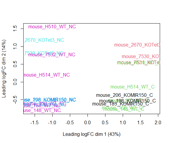
The MDS plot tells you A LOT about what to expect from your experiment.
3a. Extracting “normalized” expression table
RPKM vs. FPKM vs. CPM and Model Based
- RPKM - Reads per kilobase per million mapped reads
- FPKM - Fragments per kilobase per million mapped reads
- logCPM – log Counts per million [ good for producing MDS plots, estimate of normalized values in model based ]
- Model based - original read counts are not themselves transformed, but rather correction factors are used in the DE model itself.
We use the cpm function with log=TRUE to obtain log-transformed normalized expression data. On the log scale, the data has less mean-dependent variability and is more suitable for plotting.
logcpm <- cpm(d, prior.count=2, log=TRUE)
write.table(logcpm,"rnaseq_workshop_normalized_counts.txt",sep="\t",quote=F)
Quiz 2
4. Voom transformation and calculation of variance weights
4a. Voom
y <- voom(d, mm, plot = T)
## Coefficients not estimable: mouse206 mouse7531
## Warning: Partial NA coefficients for 11730 probe(s)
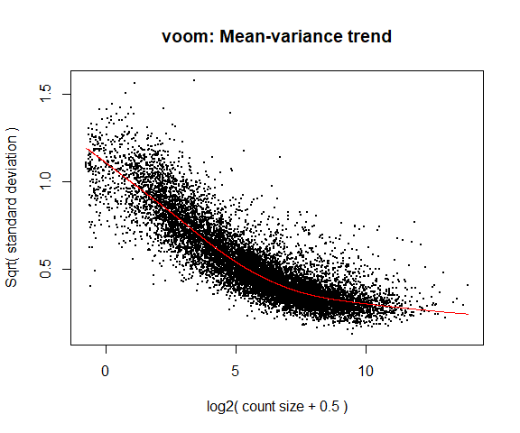
What is voom doing?
- Counts are transformed to log2 counts per million reads (CPM), where “per million reads” is defined based on the normalization factors we calculated earlier.
- A linear model is fitted to the log2 CPM for each gene, and the residuals are calculated.
- A smoothed curve is fitted to the sqrt(residual standard deviation) by average expression. (see red line in plot above)
- The smoothed curve is used to obtain weights for each gene and sample that are passed into limma along with the log2 CPMs.
More details at “voom: precision weights unlock linear model analysis tools for RNA-seq read counts”
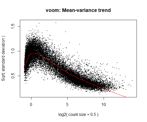
If your voom plot looks like the below (performed on the raw data), you might want to filter more:
tmp <- voom(d0, mm, plot = T)
## Coefficients not estimable: mouse206 mouse7531
## Warning: Partial NA coefficients for 78258 probe(s)
5. Fitting linear models in limma
lmFit fits a linear model using weighted least squares for each gene:
fit <- lmFit(y, mm)
## Coefficients not estimable: mouse206 mouse7531
## Warning: Partial NA coefficients for 11730 probe(s)
head(coef(fit))
##                       groupKOMIR150.C groupKOTet3.C groupWT.C groupKOMIR150.NC
## ENSMUSG00000033845.14        4.763092      4.977111  4.708462         4.951215
## ENSMUSG00000025903.15        4.970552      5.427981  5.401449         5.011436
## ENSMUSG00000033813.16        5.901702      5.679519  5.815700         5.963420
## ENSMUSG00000033793.13        5.221733      5.297331  5.426801         5.050521
## ENSMUSG00000090031.5         2.296444      3.506969  1.924746         2.446124
## ENSMUSG00000025907.15        6.374205      6.480113  6.489574         6.178288
##                       groupKOTet3.NC groupWT.NC    mouse148    mouse158
## ENSMUSG00000033845.14       4.598293   4.492926  0.23815323  0.15846864
## ENSMUSG00000025903.15       5.294709   5.142721 -0.07362720 -0.06386909
## ENSMUSG00000033813.16       5.847294   5.815173  0.04631731  0.02950469
## ENSMUSG00000033793.13       4.762922   5.135599 -0.19687120 -0.25117798
## ENSMUSG00000090031.5        3.843231   2.121721 -0.11927173  0.10737774
## ENSMUSG00000025907.15       6.539661   6.200951 -0.15011597 -0.07032668
##                          mouse183      mouse198 mouse206   mouse2670
## ENSMUSG00000033845.14 -0.34172109 -0.0510355761       NA -0.05979453
## ENSMUSG00000025903.15  0.37901419  0.3540873736       NA  0.03826178
## ENSMUSG00000033813.16 -0.22150131 -0.0007105147       NA  0.17164464
## ENSMUSG00000033793.13 -0.27459863  0.0883896936       NA  0.21318440
## ENSMUSG00000090031.5  -0.35251695  0.1651426586       NA -1.10273466
## ENSMUSG00000025907.15 -0.06077507  0.1789397004       NA -0.05099193
##                         mouse7530 mouse7531   mouse7532   mouseH510   mouseH514
## ENSMUSG00000033845.14 -0.00512802        NA  0.14083941  0.07741864  0.14396087
## ENSMUSG00000025903.15 -0.14733611        NA  0.18395490  0.12494853  0.13854630
## ENSMUSG00000033813.16  0.19565799        NA  0.06251865  0.04712923 -0.02516137
## ENSMUSG00000033793.13  0.47631353        NA -0.31871099 -0.08211622 -0.17094901
## ENSMUSG00000090031.5  -0.20420968        NA  1.89970613  1.25309299  1.45687590
## ENSMUSG00000025907.15 -0.11576758        NA  0.10885141 -0.15612992 -0.23956105
Comparisons between groups (log fold-changes) are obtained as contrasts of these fitted linear models:
6. Specify which groups to compare using contrasts:
Comparison between cell types for genotype WT.
contr <- makeContrasts(groupWT.C - groupWT.NC, levels = colnames(coef(fit)))
contr
##                   Contrasts
## Levels             groupWT.C - groupWT.NC
##   groupKOMIR150.C                       0
##   groupKOTet3.C                         0
##   groupWT.C                             1
##   groupKOMIR150.NC                      0
##   groupKOTet3.NC                        0
##   groupWT.NC                           -1
##   mouse148                              0
##   mouse158                              0
##   mouse183                              0
##   mouse198                              0
##   mouse206                              0
##   mouse2670                             0
##   mouse7530                             0
##   mouse7531                             0
##   mouse7532                             0
##   mouseH510                             0
##   mouseH514                             0
6a. Estimate contrast for each gene
tmp <- contrasts.fit(fit, contr)
The variance characteristics of low expressed genes are different from high expressed genes, if treated the same, the effect is to over represent low expressed genes in the DE list. This is corrected for by the log transformation and voom. However, some genes will have increased or decreased variance that is not a result of low expression, but due to other random factors. We are going to run empirical Bayes to adjust the variance of these genes.
Empirical Bayes smoothing of standard errors (shifts standard errors that are much larger or smaller than those from other genes towards the average standard error) (see “Linear Models and Empirical Bayes Methods for Assessing Differential Expression in Microarray Experiments”
6b. Apply EBayes
tmp <- eBayes(tmp)
7. Multiple Testing Adjustment
The TopTable. Adjust for multiple testing using method of Benjamini & Hochberg (BH), or its ‘alias’ fdr. “Controlling the false discovery rate: a practical and powerful approach to multiple testing.
here n=Inf says to produce the topTable for all genes.
top.table <- topTable(tmp, adjust.method = "BH", sort.by = "P", n = Inf)
Multiple Testing Correction
Simply a must! Best choices are:
The FDR (or qvalue) is a statement about the list and is no longer about the gene (pvalue). So a FDR of 0.05, says you expect 5% false positives among the list of genes with an FDR of 0.05 or less.
The statement “Statistically significantly different” means FDR of 0.05 or less.
7a. How many DE genes are there (false discovery rate corrected)?
length(which(top.table$adj.P.Val < 0.05))
## [1] 5729
8. Check your results for confidence.
You’ve conducted an experiment, you’ve seen a phenotype. Now check which genes are most differentially expressed (show the top 50)? Look up these top genes, their description and ensure they relate to your experiment/phenotype.
head(top.table, 50)
##                           logFC   AveExpr         t      P.Value    adj.P.Val
## ENSMUSG00000020608.8  -2.474865  7.866786 -44.34836 5.518511e-19 6.473214e-15
## ENSMUSG00000052212.7   4.558642  6.221681  40.72759 2.310858e-18 1.355318e-14
## ENSMUSG00000049103.15  2.171072  9.909926  39.08710 4.609451e-18 1.802295e-14
## ENSMUSG00000030203.18 -4.109923  7.023672 -33.69246 5.554266e-17 1.628789e-13
## ENSMUSG00000021990.17 -2.668725  8.377409 -32.93133 8.138953e-17 1.662702e-13
## ENSMUSG00000027508.16 -1.888581  8.141405 -32.84480 8.504872e-17 1.662702e-13
## ENSMUSG00000024164.16  1.807622  9.895068  32.14372 1.219693e-16 2.043857e-13
## ENSMUSG00000037820.16 -4.160120  7.139673 -31.64894 1.580384e-16 2.253566e-13
## ENSMUSG00000026193.16  4.813375 10.169379  31.47893 1.729079e-16 2.253566e-13
## ENSMUSG00000030342.9  -3.669411  6.066558 -30.23313 3.391389e-16 3.978099e-13
## ENSMUSG00000048498.9  -5.784074  6.530544 -30.02629 3.802576e-16 4.054929e-13
## ENSMUSG00000038807.20 -1.553448  9.034893 -29.61681 4.780203e-16 4.504773e-13
## ENSMUSG00000021614.17  5.996912  5.453976  29.40610 5.383919e-16 4.504773e-13
## ENSMUSG00000051177.17  3.199356  5.015169  29.38849 5.437898e-16 4.504773e-13
## ENSMUSG00000030413.8  -2.598834  6.657186 -29.28694 5.760579e-16 4.504773e-13
## ENSMUSG00000037185.10 -1.527107  9.503392 -28.93689 7.037368e-16 4.673184e-13
## ENSMUSG00000029254.17 -2.385559  6.432083 -28.89562 7.206552e-16 4.673184e-13
## ENSMUSG00000028885.9  -2.344597  7.075607 -28.88328 7.257935e-16 4.673184e-13
## ENSMUSG00000027215.14 -2.565359  6.922592 -28.81043 7.569522e-16 4.673184e-13
## ENSMUSG00000020437.13 -1.191531 10.243418 -28.62262 8.439806e-16 4.949946e-13
## ENSMUSG00000018168.9  -3.891090  5.411374 -28.49077 9.113648e-16 5.090624e-13
## ENSMUSG00000039959.14 -1.472679  8.954786 -28.10195 1.145357e-15 5.618861e-13
## ENSMUSG00000038147.15  1.697589  7.170310  28.10098 1.146013e-15 5.618861e-13
## ENSMUSG00000020108.5  -2.038446  6.975102 -28.03253 1.193437e-15 5.618861e-13
## ENSMUSG00000023827.9  -2.136703  6.433839 -28.02674 1.197541e-15 5.618861e-13
## ENSMUSG00000022584.15  4.733558  6.762779  27.65412 1.495885e-15 6.748741e-13
## ENSMUSG00000020212.15 -2.155969  6.803931 -27.46394 1.677597e-15 6.990942e-13
## ENSMUSG00000023809.12 -3.185953  4.816264 -27.42488 1.717728e-15 6.990942e-13
## ENSMUSG00000021728.9   1.677607  8.386702  27.41469 1.728366e-15 6.990942e-13
## ENSMUSG00000020387.16 -4.922221  4.358045 -27.09252 2.103227e-15 8.223619e-13
## ENSMUSG00000035493.11  1.929852  9.778559  26.63310 2.793500e-15 1.057024e-12
## ENSMUSG00000018001.19 -2.603455  7.200098 -26.54451 2.952241e-15 1.059686e-12
## ENSMUSG00000020272.9  -1.289552 10.475447 -26.52888 2.981213e-15 1.059686e-12
## ENSMUSG00000044783.17 -1.721442  7.015949 -26.21576 3.629906e-15 1.234399e-12
## ENSMUSG00000026923.16  2.013507  6.644579  26.19272 3.683202e-15 1.234399e-12
## ENSMUSG00000008496.20 -1.474004  9.434807 -25.76304 4.844602e-15 1.569003e-12
## ENSMUSG00000042700.17 -1.812531  6.104103 -25.72360 4.969109e-15 1.569003e-12
## ENSMUSG00000039109.18  4.751471  8.313540  25.68110 5.107068e-15 1.569003e-12
## ENSMUSG00000043263.14  1.796085  7.860235  25.64820 5.216633e-15 1.569003e-12
## ENSMUSG00000033705.18  1.701745  7.145382  25.41083 6.084819e-15 1.784373e-12
## ENSMUSG00000029287.15 -3.770226  5.431013 -25.15771 7.181206e-15 2.054525e-12
## ENSMUSG00000051457.8  -2.252719  9.823069 -25.03071 7.808328e-15 2.180755e-12
## ENSMUSG00000050335.18  1.119943  8.990381  24.88724 8.587041e-15 2.342465e-12
## ENSMUSG00000027435.9   3.043910  6.747184  24.76187 9.334861e-15 2.488589e-12
## ENSMUSG00000022818.14 -1.738950  6.809345 -24.41714 1.176861e-14 3.067685e-12
## ENSMUSG00000005800.4   5.743029  4.151454  24.32195 1.255293e-14 3.200997e-12
## ENSMUSG00000016496.8  -3.551720  6.431429 -24.26493 1.304907e-14 3.256715e-12
## ENSMUSG00000040809.11  3.894182  7.186954  24.07248 1.488258e-14 3.618674e-12
## ENSMUSG00000032035.17 -4.382722  5.194562 -24.04976 1.511637e-14 3.618674e-12
## ENSMUSG00000020340.17 -2.243993  8.677094 -23.81577 1.776301e-14 4.085560e-12
##                              B
## ENSMUSG00000020608.8  33.76494
## ENSMUSG00000052212.7  31.83593
## ENSMUSG00000049103.15 31.74056
## ENSMUSG00000030203.18 29.18337
## ENSMUSG00000021990.17 28.87810
## ENSMUSG00000027508.16 28.83508
## ENSMUSG00000024164.16 28.41808
## ENSMUSG00000037820.16 28.14188
## ENSMUSG00000026193.16 28.03809
## ENSMUSG00000030342.9  27.27216
## ENSMUSG00000048498.9  26.95815
## ENSMUSG00000038807.20 27.06047
## ENSMUSG00000021614.17 25.72228
## ENSMUSG00000051177.17 26.51906
## ENSMUSG00000030413.8  26.92154
## ENSMUSG00000037185.10 26.63920
## ENSMUSG00000029254.17 26.68588
## ENSMUSG00000028885.9  26.69594
## ENSMUSG00000027215.14 26.64972
## ENSMUSG00000020437.13 26.39939
## ENSMUSG00000018168.9  26.24544
## ENSMUSG00000039959.14 26.16372
## ENSMUSG00000038147.15 26.23639
## ENSMUSG00000020108.5  26.18598
## ENSMUSG00000023827.9  26.18622
## ENSMUSG00000022584.15 25.94941
## ENSMUSG00000020212.15 25.86121
## ENSMUSG00000023809.12 25.40968
## ENSMUSG00000021728.9  25.77945
## ENSMUSG00000020387.16 24.13400
## ENSMUSG00000035493.11 25.20824
## ENSMUSG00000018001.19 25.28574
## ENSMUSG00000020272.9  25.07734
## ENSMUSG00000044783.17 25.08335
## ENSMUSG00000026923.16 25.07118
## ENSMUSG00000008496.20 24.65239
## ENSMUSG00000042700.17 24.77166
## ENSMUSG00000039109.18 24.69170
## ENSMUSG00000043263.14 24.66858
## ENSMUSG00000033705.18 24.54795
## ENSMUSG00000029287.15 24.31772
## ENSMUSG00000051457.8  24.13188
## ENSMUSG00000050335.18 24.09596
## ENSMUSG00000027435.9  24.14954
## ENSMUSG00000022818.14 23.90056
## ENSMUSG00000005800.4  21.87219
## ENSMUSG00000016496.8  23.80318
## ENSMUSG00000040809.11 23.66621
## ENSMUSG00000032035.17 23.44954
## ENSMUSG00000020340.17 23.37418
Columns are
- logFC: log2 fold change of WT.C/WT.NC
- AveExpr: Average expression across all samples, in log2 CPM
- t: logFC divided by its standard error
- P.Value: Raw p-value (based on t) from test that logFC differs from 0
- adj.P.Val: Benjamini-Hochberg false discovery rate adjusted p-value
- B: log-odds that gene is DE (arguably less useful than the other columns)
ENSMUSG00000030203.18 has higher expression at WT NC than at WT C (logFC is negative). ENSMUSG00000026193.16 has higher expression at WT C than at WT NC (logFC is positive).
9. Write top.table to a file, adding in cpms and annotation
top.table$Gene <- rownames(top.table)
top.table <- top.table[,c("Gene", names(top.table)[1:6])]
top.table <- data.frame(top.table,anno[match(top.table$Gene,anno$Gene.stable.ID.version),],logcpm[match(top.table$Gene,rownames(logcpm)),])

head(top.table)
##                                        Gene     logFC  AveExpr         t
## ENSMUSG00000020608.8   ENSMUSG00000020608.8 -2.474865 7.866786 -44.34836
## ENSMUSG00000052212.7   ENSMUSG00000052212.7  4.558642 6.221681  40.72759
## ENSMUSG00000049103.15 ENSMUSG00000049103.15  2.171072 9.909926  39.08710
## ENSMUSG00000030203.18 ENSMUSG00000030203.18 -4.109923 7.023672 -33.69246
## ENSMUSG00000021990.17 ENSMUSG00000021990.17 -2.668725 8.377409 -32.93133
## ENSMUSG00000027508.16 ENSMUSG00000027508.16 -1.888581 8.141405 -32.84480
##                            P.Value    adj.P.Val        B     Gene.stable.ID
## ENSMUSG00000020608.8  5.518511e-19 6.473214e-15 33.76494 ENSMUSG00000020608
## ENSMUSG00000052212.7  2.310858e-18 1.355318e-14 31.83593 ENSMUSG00000052212
## ENSMUSG00000049103.15 4.609451e-18 1.802295e-14 31.74056 ENSMUSG00000049103
## ENSMUSG00000030203.18 5.554266e-17 1.628789e-13 29.18337 ENSMUSG00000030203
## ENSMUSG00000021990.17 8.138953e-17 1.662702e-13 28.87810 ENSMUSG00000021990
## ENSMUSG00000027508.16 8.504872e-17 1.662702e-13 28.83508 ENSMUSG00000027508
##                       Gene.stable.ID.version
## ENSMUSG00000020608.8    ENSMUSG00000020608.8
## ENSMUSG00000052212.7    ENSMUSG00000052212.7
## ENSMUSG00000049103.15  ENSMUSG00000049103.15
## ENSMUSG00000030203.18  ENSMUSG00000030203.18
## ENSMUSG00000021990.17  ENSMUSG00000021990.17
## ENSMUSG00000027508.16  ENSMUSG00000027508.16
##                                                                                                          Gene.description
## ENSMUSG00000020608.8                          structural maintenance of chromosomes 6 [Source:MGI Symbol;Acc:MGI:1914491]
## ENSMUSG00000052212.7                                                    CD177 antigen [Source:MGI Symbol;Acc:MGI:1916141]
## ENSMUSG00000049103.15                                   C-C motif chemokine receptor 2 [Source:MGI Symbol;Acc:MGI:106185]
## ENSMUSG00000030203.18                                 dual specificity phosphatase 16 [Source:MGI Symbol;Acc:MGI:1917936]
## ENSMUSG00000021990.17                                    spermatogenesis associated 13 [Source:MGI Symbol;Acc:MGI:104838]
## ENSMUSG00000027508.16 phosphoprotein associated with glycosphingolipid microdomains 1 [Source:MGI Symbol;Acc:MGI:2443160]
##                       Gene.name mouse_110_WT_C mouse_110_WT_NC mouse_148_WT_C
## ENSMUSG00000020608.8       Smc6       6.651904        9.074018       7.063397
## ENSMUSG00000052212.7      Cd177       8.658433        4.183675       8.400820
## ENSMUSG00000049103.15      Ccr2      10.941017        8.849074      11.287362
## ENSMUSG00000030203.18    Dusp16       5.041179        9.000487       5.229337
## ENSMUSG00000021990.17   Spata13       7.000397        9.570003       7.373554
## ENSMUSG00000027508.16      Pag1       7.220819        9.048607       7.093831
##                       mouse_148_WT_NC mouse_158_WT_C mouse_158_WT_NC
## ENSMUSG00000020608.8         9.410804       6.780160        9.174968
## ENSMUSG00000052212.7         3.655826       8.150458        3.412010
## ENSMUSG00000049103.15        8.980688      11.103960        8.745455
## ENSMUSG00000030203.18        9.101338       5.495884        9.222336
## ENSMUSG00000021990.17        9.797624       7.056301        9.742120
## ENSMUSG00000027508.16        9.137062       7.425959        9.281038
##                       mouse_183_KOMIR150_C mouse_183_KOMIR150_NC
## ENSMUSG00000020608.8              6.816191              9.295607
## ENSMUSG00000052212.7              8.757043              3.544603
## ENSMUSG00000049103.15            11.070790              8.743009
## ENSMUSG00000030203.18             5.251592              8.920139
## ENSMUSG00000021990.17             7.452112              9.588178
## ENSMUSG00000027508.16             7.224881              8.841999
##                       mouse_198_KOMIR150_C mouse_198_KOMIR150_NC
## ENSMUSG00000020608.8              6.527885              8.981758
## ENSMUSG00000052212.7              8.679985              3.785408
## ENSMUSG00000049103.15            10.747693              8.533035
## ENSMUSG00000030203.18             4.825248              9.211816
## ENSMUSG00000021990.17             6.576745              9.329835
## ENSMUSG00000027508.16             7.073161              8.814120
##                       mouse_206_KOMIR150_C mouse_206_KOMIR150_NC
## ENSMUSG00000020608.8              6.415268              8.918616
## ENSMUSG00000052212.7              8.763092              3.659552
## ENSMUSG00000049103.15            10.799952              8.535038
## ENSMUSG00000030203.18             5.246865              9.503852
## ENSMUSG00000021990.17             6.589159              9.176432
## ENSMUSG00000027508.16             6.945408              8.863026
##                       mouse_2670_KOTet3_C mouse_2670_KOTet3_NC
## ENSMUSG00000020608.8             6.562165             9.510447
## ENSMUSG00000052212.7             7.849558             4.122247
## ENSMUSG00000049103.15           11.479697             7.544854
## ENSMUSG00000030203.18            4.969492             9.905548
## ENSMUSG00000021990.17            7.807240            10.638090
## ENSMUSG00000027508.16            7.754293             9.502032
##                       mouse_7530_KOTet3_C mouse_7530_KOTet3_NC
## ENSMUSG00000020608.8             6.421885             9.340020
## ENSMUSG00000052212.7             8.264054             3.313715
## ENSMUSG00000049103.15           11.212022             7.239365
## ENSMUSG00000030203.18            4.070243             9.475139
## ENSMUSG00000021990.17            7.352625            10.457166
## ENSMUSG00000027508.16            7.453258             9.439871
##                       mouse_7531_KOTet3_C mouse_7532_WT_NC mouse_H510_WT_C
## ENSMUSG00000020608.8             6.277701         8.845438        6.441870
## ENSMUSG00000052212.7             9.041948         4.559088        8.967768
## ENSMUSG00000049103.15           11.347131         9.603722       11.454860
## ENSMUSG00000030203.18            4.104450         9.028812        4.178293
## ENSMUSG00000021990.17            6.916742         9.527685        6.522529
## ENSMUSG00000027508.16            7.354796         8.960182        6.835884
##                       mouse_H510_WT_NC mouse_H514_WT_C mouse_H514_WT_NC
## ENSMUSG00000020608.8          8.995935        6.508879         9.169496
## ENSMUSG00000052212.7          4.612915        8.792855         4.361021
## ENSMUSG00000049103.15         9.544756       11.248271         9.036455
## ENSMUSG00000030203.18         9.038232        4.876668         9.194502
## ENSMUSG00000021990.17         9.461903        6.852537         9.598516
## ENSMUSG00000027508.16         8.693900        7.198316         9.028988
write.table(top.table, file = "WT.C_v_WT.NC.txt", row.names = F, sep = "\t", quote = F)
Quiz 3
Linear models and contrasts
Let’s say we want to compare genotypes for cell type C. The only thing we have to change is the call to makeContrasts:
contr <- makeContrasts(groupWT.C - groupKOMIR150.C, levels = colnames(coef(fit)))
tmp <- contrasts.fit(fit, contr)
tmp <- eBayes(tmp)
top.table <- topTable(tmp, sort.by = "P", n = Inf)
head(top.table, 20)
##                            logFC  AveExpr          t      P.Value    adj.P.Val
## ENSMUSG00000030703.9  -2.9716967 4.567089 -14.446204 5.790525e-11 6.792286e-07
## ENSMUSG00000044229.10 -3.2249767 6.860922 -11.442807 2.125096e-09 1.246369e-05
## ENSMUSG00000030748.10  1.7436993 7.080600   8.954175 7.751238e-08 2.522433e-04
## ENSMUSG00000066687.6  -2.0532818 4.955459  -8.888485 8.601648e-08 2.522433e-04
## ENSMUSG00000032012.10 -5.2192844 5.035597  -8.721504 1.123353e-07 2.635386e-04
## ENSMUSG00000040152.9  -2.2196214 6.471345  -8.547584 1.488778e-07 2.910561e-04
## ENSMUSG00000008348.10 -1.1872912 6.276497  -7.785366 5.349372e-07 8.662792e-04
## ENSMUSG00000028028.12  0.9017897 7.232652   7.727964 5.908128e-07 8.662792e-04
## ENSMUSG00000141370.1   4.6112490 3.079676   7.412523 1.027856e-06 1.339639e-03
## ENSMUSG00000020893.18 -1.2020133 7.566695  -7.029090 2.051371e-06 2.406258e-03
## ENSMUSG00000028037.14  5.6408258 2.287292   6.722704 3.614748e-06 3.416293e-03
## ENSMUSG00000055435.7  -1.3675279 4.998617  -6.711885 3.688649e-06 3.416293e-03
## ENSMUSG00000121395.2  -6.0838438 2.091902  -6.631863 4.286412e-06 3.416293e-03
## ENSMUSG00000039146.6   7.4650562 0.152343   6.623669 4.353061e-06 3.416293e-03
## ENSMUSG00000030365.12  1.0001775 6.602540   6.621769 4.368661e-06 3.416293e-03
## ENSMUSG00000028619.16  3.2154665 4.629995   6.346913 7.369474e-06 5.253976e-03
## ENSMUSG00000024772.10 -1.2789019 6.357753  -6.329900 7.614457e-06 5.253976e-03
## ENSMUSG00000051495.9  -0.8463233 7.170625  -6.069619 1.261947e-05 8.223687e-03
## ENSMUSG00000042105.19 -0.6827999 7.469612  -5.896664 1.774216e-05 1.095345e-02
## ENSMUSG00000054008.10 -0.9512147 6.590688  -5.707879 2.584987e-05 1.493897e-02
##                               B
## ENSMUSG00000030703.9  14.921781
## ENSMUSG00000044229.10 11.883492
## ENSMUSG00000030748.10  8.372413
## ENSMUSG00000066687.6   8.177787
## ENSMUSG00000032012.10  7.054184
## ENSMUSG00000040152.9   7.585865
## ENSMUSG00000008348.10  6.376564
## ENSMUSG00000028028.12  6.197467
## ENSMUSG00000141370.1   4.502802
## ENSMUSG00000020893.18  4.873984
## ENSMUSG00000028037.14  3.063695
## ENSMUSG00000055435.7   4.548589
## ENSMUSG00000121395.2   1.385596
## ENSMUSG00000039146.6   1.013048
## ENSMUSG00000030365.12  4.333990
## ENSMUSG00000028619.16  3.483991
## ENSMUSG00000024772.10  3.707554
## ENSMUSG00000051495.9   3.076110
## ENSMUSG00000042105.19  2.691159
## ENSMUSG00000054008.10  2.413960
length(which(top.table$adj.P.Val < 0.05)) # number of DE genes
## [1] 43
top.table$Gene <- rownames(top.table)
top.table <- top.table[,c("Gene", names(top.table)[1:6])]
top.table <- data.frame(top.table,anno[match(top.table$Gene,anno$Gene.stable.ID.version),],logcpm[match(top.table$Gene,rownames(logcpm)),])

write.table(top.table, file = "WT.C_v_KOMIR150.C.txt", row.names = F, sep = "\t", quote = F)
More complicated models
Specifying a different model is simply a matter of changing the calls to model.matrix (and possibly to contrasts.fit).
What if we want to adjust for a continuous variable like some health score? (We are making this data up here, but it would typically be a variable in your metadata.)
# Generate example health data
set.seed(99)
HScore <- rnorm(n = 22, mean = 7.5, sd = 1)
HScore
##  [1] 7.713963 7.979658 7.587829 7.943859 7.137162 7.622674 6.636155 7.989624
##  [9] 7.135883 6.205758 6.754231 8.421550 8.250054 4.991446 4.459066 7.500266
## [17] 7.105981 5.754972 7.998631 7.770954 8.598922 8.252513
Model adjusting for HScore score:
mm <- model.matrix(~0 + group + mouse + HScore)
y <- voom(d, mm, plot = F)
## Coefficients not estimable: mouse206 mouse7531
## Warning: Partial NA coefficients for 11730 probe(s)
fit <- lmFit(y, mm)
## Coefficients not estimable: mouse206 mouse7531
## Warning: Partial NA coefficients for 11730 probe(s)
contr <- makeContrasts(groupKOMIR150.NC - groupWT.NC,
                       levels = colnames(coef(fit)))
tmp <- contrasts.fit(fit, contr)
tmp <- eBayes(tmp)
top.table <- topTable(tmp, sort.by = "P", n = Inf)
head(top.table, 20)
##                            logFC  AveExpr         t      P.Value    adj.P.Val
## ENSMUSG00000044229.10  3.1864489 6.860922 21.186441 1.423074e-13 1.669266e-09
## ENSMUSG00000032012.10  5.4864163 5.035597 14.522780 5.965548e-11 2.732149e-07
## ENSMUSG00000030703.9   3.2985191 4.567089 14.376715 6.987594e-11 2.732149e-07
## ENSMUSG00000121395.2   5.9235229 2.091902 10.435879 9.115332e-09 2.673071e-05
## ENSMUSG00000040152.9   3.0240649 6.471345  9.904802 1.953971e-08 4.584016e-05
## ENSMUSG00000008348.10  1.3103387 6.276497  9.387617 4.226700e-08 8.263199e-05
## ENSMUSG00000028619.16 -2.9556433 4.629995 -8.748252 1.144180e-07 1.849051e-04
## ENSMUSG00000028173.11 -1.8285816 6.702552 -8.687417 1.261075e-07 1.849051e-04
## ENSMUSG00000100801.2  -2.5756286 5.614500 -8.566316 1.532572e-07 1.997453e-04
## ENSMUSG00000070372.12  0.9074018 7.440033  8.482734 1.755177e-07 2.058823e-04
## ENSMUSG00000020893.18  1.0915976 7.566695  8.413556 1.964962e-07 2.095364e-04
## ENSMUSG00000042396.11 -1.0174723 6.564696 -8.220990 2.699048e-07 2.638319e-04
## ENSMUSG00000030365.12 -1.0528049 6.602540 -8.121321 3.186845e-07 2.875515e-04
## ENSMUSG00000030748.10 -0.9972178 7.080600 -7.698579 6.539585e-07 5.479238e-04
## ENSMUSG00000035212.15  0.8049642 7.146025  7.451480 1.006319e-06 7.088820e-04
## ENSMUSG00000140457.1   1.8371693 6.309407  7.440234 1.026452e-06 7.088820e-04
## ENSMUSG00000028028.12 -0.8523944 7.232652 -7.423601 1.057003e-06 7.088820e-04
## ENSMUSG00000066687.6   1.8330551 4.955459  7.407335 1.087798e-06 7.088820e-04
## ENSMUSG00000141370.1  -3.6955570 3.079676 -6.850327 2.971552e-06 1.834542e-03
## ENSMUSG00000063065.14 -0.6391048 7.953322 -6.705095 3.888544e-06 2.280631e-03
##                               B
## ENSMUSG00000044229.10 21.140143
## ENSMUSG00000032012.10 14.226470
## ENSMUSG00000030703.9  14.494237
## ENSMUSG00000121395.2   6.527239
## ENSMUSG00000040152.9   9.724121
## ENSMUSG00000008348.10  8.903414
## ENSMUSG00000028619.16  7.550431
## ENSMUSG00000028173.11  7.837927
## ENSMUSG00000100801.2   7.699901
## ENSMUSG00000070372.12  7.350456
## ENSMUSG00000020893.18  7.238974
## ENSMUSG00000042396.11  7.048180
## ENSMUSG00000030365.12  6.939069
## ENSMUSG00000030748.10  6.100757
## ENSMUSG00000035212.15  5.641774
## ENSMUSG00000140457.1   5.779893
## ENSMUSG00000028028.12  5.610536
## ENSMUSG00000066687.6   5.779705
## ENSMUSG00000141370.1   3.682533
## ENSMUSG00000063065.14  4.160586
length(which(top.table$adj.P.Val < 0.05))
## [1] 101
What if we want to look at the correlation of gene expression with a continuous variable like pH?
# Generate example pH data
set.seed(99)
pH <- rnorm(n = 22, mean = 8, sd = 1.5)
pH
##  [1] 8.320944 8.719487 8.131743 8.665788 7.455743 8.184011 6.704232 8.734436
##  [9] 7.453825 6.058637 6.881346 9.382326 9.125082 4.237169 3.438599 8.000399
## [17] 7.408972 5.382459 8.747947 8.406431 9.648382 9.128770
Specify model matrix:
mm <- model.matrix(~pH)
head(mm)
##   (Intercept)       pH
## 1           1 8.320944
## 2           1 8.719487
## 3           1 8.131743
## 4           1 8.665788
## 5           1 7.455743
## 6           1 8.184011
y <- voom(d, mm, plot = F)
fit <- lmFit(y, mm)
tmp <- contrasts.fit(fit, coef = 2) # test "pH" coefficient
tmp <- eBayes(tmp)
top.table <- topTable(tmp, sort.by = "P", n = Inf)
head(top.table, 20)
##                             logFC    AveExpr         t      P.Value adj.P.Val
## ENSMUSG00000056054.10 -1.18956424  1.0831449 -5.146776 3.278063e-05 0.3845168
## ENSMUSG00000094497.2  -0.96308549 -0.5981730 -4.738753 9.004927e-05 0.4048421
## ENSMUSG00000026822.15 -1.15880018  1.2828841 -4.682602 1.035402e-04 0.4048421
## ENSMUSG00000027111.17 -0.51599508  2.0089103 -4.278979 2.828097e-04 0.8293394
## ENSMUSG00000069049.12 -1.17752902  1.5650130 -4.117695 4.223900e-04 0.9909269
## ENSMUSG00000056071.13 -1.00646251  0.9290471 -3.856057 8.078592e-04 0.9995148
## ENSMUSG00000069045.12 -1.22381353  2.0982422 -3.808842 9.077291e-04 0.9995148
## ENSMUSG00000120849.2  -0.78703501 -0.1225318 -3.806920 9.120427e-04 0.9995148
## ENSMUSG00000016356.19  0.26545995  1.7223015  3.594238 1.537978e-03 0.9995148
## ENSMUSG00000056673.15 -1.10367841  1.1017672 -3.573866 1.616515e-03 0.9995148
## ENSMUSG00000031843.3  -0.17541697  3.6300053 -3.519670 1.845078e-03 0.9995148
## ENSMUSG00000036764.13 -0.34937015  0.1741512 -3.484500 2.010024e-03 0.9995148
## ENSMUSG00000040521.12 -0.17363866  2.8910488 -3.482857 2.018068e-03 0.9995148
## ENSMUSG00000046032.17 -0.07751948  5.1932912 -3.471922 2.072444e-03 0.9995148
## ENSMUSG00000035877.18 -0.16468435  2.7716111 -3.459740 2.134699e-03 0.9995148
## ENSMUSG00000090946.4  -0.10063947  5.8370796 -3.400627 2.463678e-03 0.9995148
## ENSMUSG00000030835.7  -0.07788246  5.6990723 -3.399456 2.470669e-03 0.9995148
## ENSMUSG00000041747.4  -0.10888459  4.4917777 -3.398186 2.478277e-03 0.9995148
## ENSMUSG00000091537.3  -0.09109203  5.4693065 -3.397126 2.484642e-03 0.9995148
## ENSMUSG00000068457.15 -0.86985058  0.1150896 -3.340155 2.851201e-03 0.9995148
##                                B
## ENSMUSG00000056054.10  0.1742285
## ENSMUSG00000094497.2  -1.8379434
## ENSMUSG00000026822.15 -0.3354301
## ENSMUSG00000027111.17 -0.5838815
## ENSMUSG00000069049.12 -0.7597727
## ENSMUSG00000056071.13 -1.7433410
## ENSMUSG00000069045.12 -1.0648534
## ENSMUSG00000120849.2  -2.4217233
## ENSMUSG00000016356.19 -2.6741527
## ENSMUSG00000056673.15 -1.9046288
## ENSMUSG00000031843.3  -1.3549650
## ENSMUSG00000036764.13 -2.9863577
## ENSMUSG00000040521.12 -1.6423466
## ENSMUSG00000046032.17 -1.3002397
## ENSMUSG00000035877.18 -1.7186616
## ENSMUSG00000090946.4  -1.4465325
## ENSMUSG00000030835.7  -1.4477106
## ENSMUSG00000041747.4  -1.4767271
## ENSMUSG00000091537.3  -1.4516030
## ENSMUSG00000068457.15 -2.7657278
length(which(top.table$adj.P.Val < 0.05))
## [1] 0
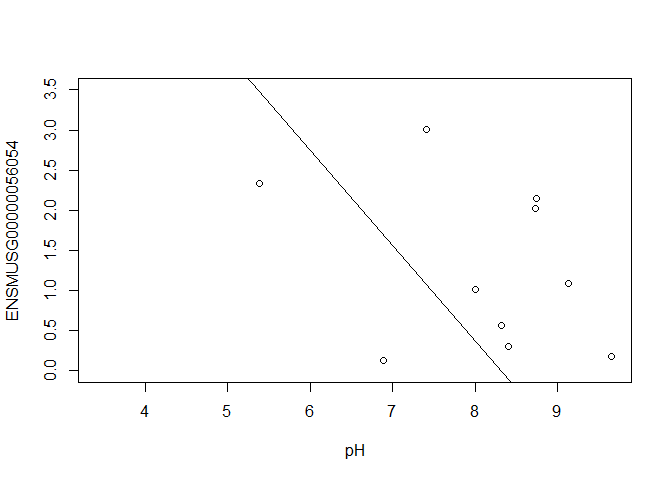
In this case, limma is fitting a linear regression model, which here is a straight line fit, with the slope and intercept defined by the model coefficients:
ENSMUSG00000056054 <- y$E["ENSMUSG00000056054.10",]
plot(ENSMUSG00000056054 ~ pH, ylim = c(0, 3.5))
intercept <- coef(fit)["ENSMUSG00000056054.10", "(Intercept)"]
slope <- coef(fit)["ENSMUSG00000056054.10", "pH"]
abline(a = intercept, b = slope)
slope
## [1] -1.189564
In this example, the log fold change logFC is the slope of the line, or the change in gene expression (on the log2 CPM scale) for each unit increase in pH.
Here, a logFC of 0.20 means a 0.20 log2 CPM increase in gene expression for each unit increase in pH, or a 15% increase on the CPM scale (2^0.20 = 1.15).
A bit more on linear models
Limma fits a linear model to each gene.
Linear models include analysis of variance (ANOVA) models, linear regression, and any model of the form
Y = β0 + β1X1 + β2X2 + … + βpXp + ε
The covariates X can be:
- a continuous variable (pH, HScore score, age, weight, temperature, etc.)
- Dummy variables coding a categorical covariate (like cell type, genotype, and group)
The β’s are unknown parameters to be estimated.
In limma, the β’s are the log fold changes.
The error (residual) term ε is assumed to be normally distributed with a variance that is constant across the range of the data.
Normally distributed means the residuals come from a distribution that looks like this:
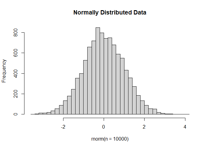
The log2 transformation that voom applies to the counts makes the data “normal enough”, but doesn’t completely stabilize the variance:
mm <- model.matrix(~0 + group + mouse)
tmp <- voom(d, mm, plot = T)
## Coefficients not estimable: mouse206 mouse7531
## Warning: Partial NA coefficients for 11730 probe(s)
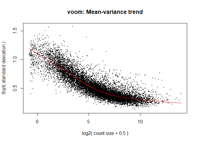
The log2 counts per million are more variable at lower expression levels. The variance weights calculated by voom address this situation.
Both edgeR and limma have VERY comprehensive user manuals
The limma users’ guide has great details on model specification.
Simple plotting
mm <- model.matrix(~0 + group + mouse)
colnames(mm) <- make.names(colnames(mm))
y <- voom(d, mm, plot = F)
## Coefficients not estimable: mouse206 mouse7531
## Warning: Partial NA coefficients for 11730 probe(s)
fit <- lmFit(y, mm)
## Coefficients not estimable: mouse206 mouse7531
## Warning: Partial NA coefficients for 11730 probe(s)
contrast.matrix <- makeContrasts(groupKOMIR150.C - groupWT.C, levels=colnames(coef(fit)))
fit2 <- contrasts.fit(fit, contrast.matrix)
fit2 <- eBayes(fit2)
top.table <- topTable(fit2, coef = 1, sort.by = "P", n = 40)
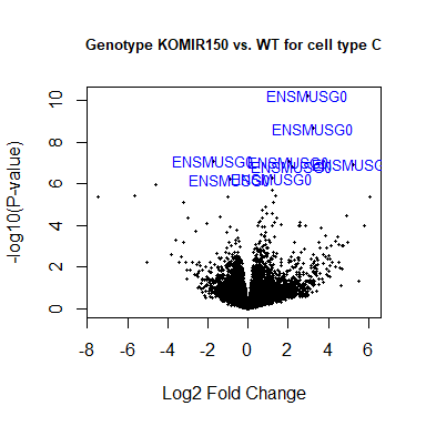
Volcano plot
volcanoplot(fit2, coef=1, highlight=8, names=rownames(fit2), main="Genotype KOMIR150 vs. WT for cell type C", cex.main = 0.8)
head(anno[match(rownames(fit2), anno$Gene.stable.ID.version),
     c("Gene.stable.ID.version", "Gene.name") ])
##       Gene.stable.ID.version     Gene.name
## 38959  ENSMUSG00000033845.14        Mrpl15
## 39236  ENSMUSG00000025903.15        Lypla1
## 39617  ENSMUSG00000033813.16         Tcea1
## 40878  ENSMUSG00000033793.13       Atp6v1h
## 65524   ENSMUSG00000090031.5 4732440D04Rik
## 41377  ENSMUSG00000025907.15        Rb1cc1
identical(anno[match(rownames(fit2), anno$Gene.stable.ID.version),
     c("Gene.stable.ID.version")], rownames(fit2))
## [1] TRUE
volcanoplot(fit2, coef=1, highlight=8, names=anno[match(rownames(fit2), anno$Gene.stable.ID.version), "Gene.name"], main="Genotype KOMIR150 vs. WT for cell type C", cex.main = 0.8)

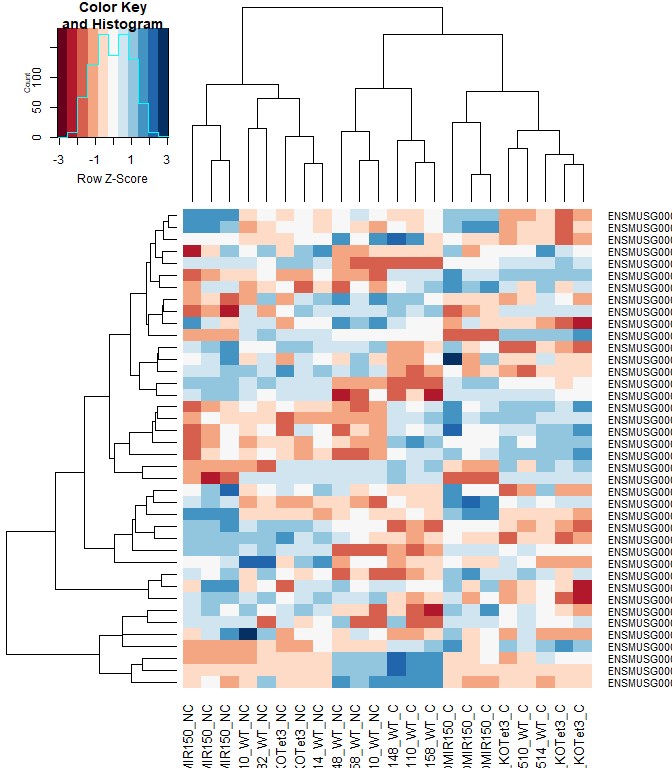
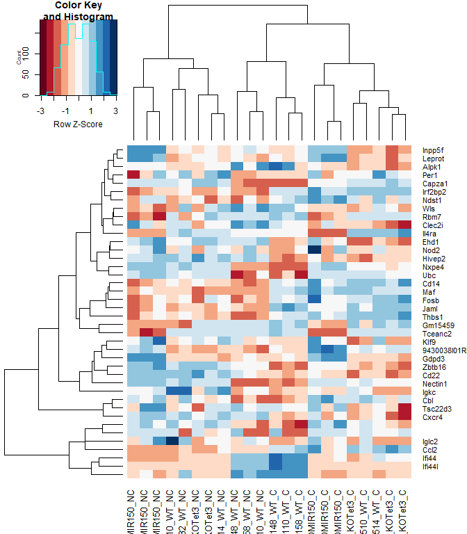
Heatmap
#using a red and blue color scheme without traces and scaling each row
heatmap.2(logcpm[rownames(top.table),],col=brewer.pal(11,"RdBu"),scale="row", trace="none")
anno[match(rownames(top.table), anno$Gene.stable.ID.version),
     c("Gene.stable.ID.version", "Gene.name")]
##       Gene.stable.ID.version     Gene.name
## 55627   ENSMUSG00000030703.9         Gdpd3
## 67823  ENSMUSG00000044229.10         Nxpe4
## 67418  ENSMUSG00000030748.10         Il4ra
## 67906   ENSMUSG00000066687.6        Zbtb16
## 16402  ENSMUSG00000032012.10       Nectin1
## 49815   ENSMUSG00000040152.9         Thbs1
## 22876  ENSMUSG00000008348.10           Ubc
## 13138  ENSMUSG00000028028.12         Alpk1
## 68303   ENSMUSG00000141370.1
## 65762  ENSMUSG00000020893.18          Per1
## 2080   ENSMUSG00000028037.14         Ifi44
## 14891   ENSMUSG00000055435.7           Maf
## 49839   ENSMUSG00000121395.2
## 2101    ENSMUSG00000039146.6        Ifi44l
## 46318  ENSMUSG00000030365.12        Clec2i
## 6183   ENSMUSG00000028619.16       Tceanc2
## 33235  ENSMUSG00000024772.10          Ehd1
## 23607   ENSMUSG00000051495.9       Irf2bp2
## 65406  ENSMUSG00000042105.19        Inpp5f
## 21760  ENSMUSG00000054008.10         Ndst1
## 17327  ENSMUSG00000055994.16          Nod2
## 12649   ENSMUSG00000076937.4         Iglc2
## 11965  ENSMUSG00000028173.11           Wls
## 688     ENSMUSG00000033863.3          Klf9
## 67063   ENSMUSG00000100801.2       Gm15459
## 25814  ENSMUSG00000070372.12        Capza1
## 24366  ENSMUSG00000035212.15        Leprot
## 12323  ENSMUSG00000031431.14       Tsc22d3
## 64589   ENSMUSG00000035385.6          Ccl2
## 24024   ENSMUSG00000051439.8          Cd14
## 53346   ENSMUSG00000048534.8          Jaml
## 65581  ENSMUSG00000040139.15 9430038I01Rik
## 55645   ENSMUSG00000141229.1
## 15414   ENSMUSG00000003545.4          Fosb
## 18191  ENSMUSG00000034342.10           Cbl
## 68883  ENSMUSG00000030577.15          Cd22
## 4950    ENSMUSG00000076609.3          Igkc
## 23958  ENSMUSG00000015501.11        Hivep2
## 18249   ENSMUSG00000045382.7         Cxcr4
## 67885  ENSMUSG00000042396.11          Rbm7
identical(anno[match(rownames(top.table), anno$Gene.stable.ID.version), "Gene.stable.ID.version"], rownames(top.table))
## [1] TRUE
heatmap.2(logcpm[rownames(top.table),],col=brewer.pal(11,"RdBu"),scale="row", trace="none", labRow = anno[match(rownames(top.table), anno$Gene.stable.ID.version), "Gene.name"])
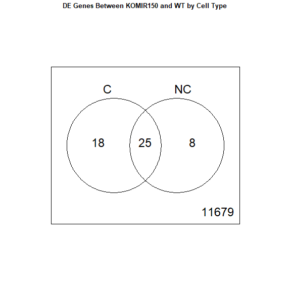
2 factor venn diagram
mm <- model.matrix(~0 + group + mouse)
colnames(mm) <- make.names(colnames(mm))
y <- voom(d, mm, plot = F)
## Coefficients not estimable: mouse206 mouse7531
## Warning: Partial NA coefficients for 11730 probe(s)
fit <- lmFit(y, mm)
## Coefficients not estimable: mouse206 mouse7531
## Warning: Partial NA coefficients for 11730 probe(s)
contrast.matrix <- makeContrasts(groupKOMIR150.C - groupWT.C, groupKOMIR150.NC - groupWT.NC, levels=colnames(coef(fit)))
fit2 <- contrasts.fit(fit, contrast.matrix)
fit2 <- eBayes(fit2)
top.table <- topTable(fit2, coef = 1, sort.by = "P", n = 40)

results <- decideTests(fit2)
vennDiagram(results, names = c("C", "NC"), main = "DE Genes Between KOMIR150 and WT by Cell Type", cex.main = 0.8)
Download the Enrichment Analysis R Markdown document
download.file("https://raw.githubusercontent.com/ucdavis-bioinformatics-training/2024-June-RNA-Seq-Analysis/master/data_analysis/enrichment_mm.Rmd", "enrichment_mm.Rmd")
sessionInfo()
## R version 4.5.0 (2025-04-11 ucrt)
## Platform: x86_64-w64-mingw32/x64
## Running under: Windows 11 x64 (build 26100)
##
## Matrix products: default
##   LAPACK version 3.12.1
##
## locale:
## [1] LC_COLLATE=English_United States.utf8
## [2] LC_CTYPE=English_United States.utf8
## [3] LC_MONETARY=English_United States.utf8
## [4] LC_NUMERIC=C
## [5] LC_TIME=English_United States.utf8
##
## time zone: America/Los_Angeles
## tzcode source: internal
##
## attached base packages:
## [1] stats     graphics  grDevices utils     datasets  methods   base
##
## other attached packages:
## [1] gplots_3.2.0       RColorBrewer_1.1-3 edgeR_4.6.2        limma_3.64.1
##
## loaded via a namespace (and not attached):
##  [1] cli_3.6.5          knitr_1.50         rlang_1.1.6        xfun_0.52
##  [5] KernSmooth_2.23-26 jsonlite_2.0.0     gtools_3.9.5       statmod_1.5.0
##  [9] htmltools_0.5.8.1  sass_0.4.10        locfit_1.5-9.12    rmarkdown_2.29
## [13] grid_4.5.0         evaluate_1.0.3     jquerylib_0.1.4    caTools_1.18.3
## [17] bitops_1.0-9       fastmap_1.2.0      yaml_2.3.10        lifecycle_1.0.4
## [21] compiler_4.5.0     lattice_0.22-7     digest_0.6.37      R6_2.6.1
## [25] bslib_0.9.0        tools_4.5.0        cachem_1.1.0