
GO AND KEGG Enrichment Analysis
Load libraries
library(topGO)
library(org.Mm.eg.db)
library(clusterProfiler)
library(pathview)
library(enrichplot)
library(ggplot2)
library(dplyr)
Files for examples were created in the DE analysis.
Gene Ontology (GO) Enrichment
Gene ontology provides a controlled vocabulary for describing biological processes (BP ontology), molecular functions (MF ontology) and cellular components (CC ontology)
The GO ontologies themselves are organism-independent; terms are associated with genes for a specific organism through direct experimentation or through sequence homology with another organism and its GO annotation.
Terms are related to other terms through parent-child relationships in a directed acylic graph.
Enrichment analysis provides one way of drawing conclusions about a set of differential expression results.
1. topGO Example Using Kolmogorov-Smirnov Testing Our first example uses Kolmogorov-Smirnov Testing for enrichment testing of our mouse DE results, with GO annotation obtained from the Bioconductor database org.Mm.eg.db.
The first step in each topGO analysis is to create a topGOdata object. This contains the genes, the score for each gene (here we use the p-value from the DE test), the GO terms associated with each gene, and the ontology to be used (here we use the biological process ontology)
infile <- "WT.C_v_WT.NC.txt"
DE <- read.delim(infile)

## Add entrezgene IDs to top table
tmp <- bitr(DE$Gene.stable.ID, fromType = "ENSEMBL", toType = "ENTREZID", OrgDb = org.Mm.eg.db)
## 'select()' returned 1:many mapping between keys and columns
## Warning in bitr(DE$Gene.stable.ID, fromType = "ENSEMBL", toType = "ENTREZID", :
## 6.93% of input gene IDs are fail to map...
id.conv <- subset(tmp, !duplicated(tmp$ENSEMBL))
DE <- left_join(DE, id.conv, by = c("Gene.stable.ID" = "ENSEMBL"))

# Make gene list
DE.nodupENTREZ <- subset(DE, !is.na(ENTREZID) & !duplicated(ENTREZID))
geneList <- DE.nodupENTREZ$P.Value
names(geneList) <- DE.nodupENTREZ$ENTREZID
head(geneList)
##        67241        68891        12772        70686       219140        94212
## 5.518511e-19 2.310858e-18 4.609451e-18 5.554266e-17 8.138953e-17 8.504872e-17
# Create topGOData object
GOdata <- new("topGOdata",
	ontology = "BP",
	allGenes = geneList,
	geneSelectionFun = function(x)x,
	annot = annFUN.org , mapping = "org.Mm.eg.db")
##
## Building most specific GOs .....
## ( 10608 GO terms found. )
##
## Build GO DAG topology ..........
## ( 13703 GO terms and 30140 relations. )
##
## Annotating nodes ...............
## ( 10477 genes annotated to the GO terms. )
2. The topGOdata object is then used as input for enrichment testing:
# Kolmogorov-Smirnov testing
resultKS <- runTest(GOdata, algorithm = "weight01", statistic = "ks")
##
## 			 -- Weight01 Algorithm --
##
## 		 the algorithm is scoring 13703 nontrivial nodes
## 		 parameters:
## 			 test statistic: ks
## 			 score order: increasing
##
## 	 Level 19:	2 nodes to be scored	(0 eliminated genes)
##
## 	 Level 18:	25 nodes to be scored	(0 eliminated genes)
##
## 	 Level 17:	51 nodes to be scored	(39 eliminated genes)
##
## 	 Level 16:	92 nodes to be scored	(108 eliminated genes)
##
## 	 Level 15:	127 nodes to be scored	(209 eliminated genes)
##
## 	 Level 14:	245 nodes to be scored	(473 eliminated genes)
##
## 	 Level 13:	564 nodes to be scored	(839 eliminated genes)
##
## 	 Level 12:	1010 nodes to be scored	(1422 eliminated genes)
##
## 	 Level 11:	1548 nodes to be scored	(2566 eliminated genes)
##
## 	 Level 10:	1817 nodes to be scored	(4354 eliminated genes)
##
## 	 Level 9:	2013 nodes to be scored	(6008 eliminated genes)
##
## 	 Level 8:	1909 nodes to be scored	(7351 eliminated genes)
##
## 	 Level 7:	1666 nodes to be scored	(8220 eliminated genes)
##
## 	 Level 6:	1324 nodes to be scored	(8898 eliminated genes)
##
## 	 Level 5:	812 nodes to be scored	(9267 eliminated genes)
##
## 	 Level 4:	376 nodes to be scored	(9503 eliminated genes)
##
## 	 Level 3:	104 nodes to be scored	(9628 eliminated genes)
##
## 	 Level 2:	17 nodes to be scored	(9656 eliminated genes)
##
## 	 Level 1:	1 nodes to be scored	(9703 eliminated genes)
tab <- GenTable(GOdata, raw.p.value = resultKS, topNodes = length(resultKS@score), numChar = 120)
topGO by default preferentially tests more specific terms, utilizing the topology of the GO graph. The algorithms used are described in detail here.
head(tab, 15)
##         GO.ID
## 1  GO:0045944
## 2  GO:0045071
## 3  GO:0032760
## 4  GO:0032731
## 5  GO:0001525
## 6  GO:0035458
## 7  GO:0045766
## 8  GO:0070374
## 9  GO:0006002
## 10 GO:0045087
## 11 GO:0035556
## 12 GO:0140242
## 13 GO:0032956
## 14 GO:0051897
## 15 GO:0140236
##                                                                                         Term
## 1                                  positive regulation of transcription by RNA polymerase II
## 2                                            negative regulation of viral genome replication
## 3                                    positive regulation of tumor necrosis factor production
## 4                                       positive regulation of interleukin-1 beta production
## 5                                                                               angiogenesis
## 6                                                       cellular response to interferon-beta
## 7                                                        positive regulation of angiogenesis
## 8                                               positive regulation of ERK1 and ERK2 cascade
## 9                                                     fructose 6-phosphate metabolic process
## 10                                                                    innate immune response
## 11                                                         intracellular signal transduction
## 12                                                                translation at postsynapse
## 13                                             regulation of actin cytoskeleton organization
## 14 positive regulation of phosphatidylinositol 3-kinase/protein kinase B signal transduction
## 15                                                                 translation at presynapse
##    Annotated Significant Expected raw.p.value
## 1        800         800      800     6.1e-09
## 2         51          51       51     2.5e-08
## 3         97          97       97     7.9e-08
## 4         54          54       54     1.5e-07
## 5        324         324      324     2.9e-07
## 6         54          54       54     3.4e-07
## 7         99          99       99     4.2e-07
## 8        103         103      103     1.8e-06
## 9         12          12       12     2.9e-06
## 10       708         708      708     5.2e-06
## 11      1971        1971     1971     5.9e-06
## 12        46          46       46     8.1e-06
## 13       230         230      230     9.3e-06
## 14       103         103      103     1.2e-05
## 15        45          45       45     1.2e-05
- Annotated: number of genes (in our gene list) that are annotated with the term
- Significant: n/a for this example, same as Annotated here
- Expected: n/a for this example, same as Annotated here
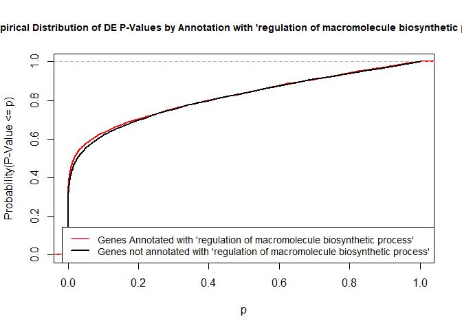
- raw.p.value: P-value from Kolomogorov-Smirnov test that DE p-values annotated with the term are smaller (i.e. more significant) than those not annotated with the term.
The Kolmogorov-Smirnov test directly compares two probability distributions based on their maximum distance.
To illustrate the KS test, we plot probability distributions of p-values that are and that are not annotated with the term GO:0010556 “regulation of macromolecule biosynthetic process” (2344 genes) p-value 1.00. (This won’t exactly match what topGO does due to their elimination algorithm):
rna.pp.terms <- genesInTerm(GOdata)[["GO:0010556"]] # get genes associated with term
p.values.in <- geneList[names(geneList) %in% rna.pp.terms]
p.values.out <- geneList[!(names(geneList) %in% rna.pp.terms)]
plot.ecdf(p.values.in, verticals = T, do.points = F, col = "red", lwd = 2, xlim = c(0,1),
          main = "Empirical Distribution of DE P-Values by Annotation with 'regulation of macromolecule biosynthetic process'",
          cex.main = 0.9, xlab = "p", ylab = "Probability(P-Value <= p)")
ecdf.out <- ecdf(p.values.out)
xx <- unique(sort(c(seq(0, 1, length = 201), knots(ecdf.out))))
lines(xx, ecdf.out(xx), col = "black", lwd = 2)
legend("bottomright", legend = c("Genes Annotated with 'regulation of macromolecule biosynthetic process'", "Genes not annotated with 'regulation of macromolecule biosynthetic process'"), lwd = 2, col = 2:1, cex = 0.9)
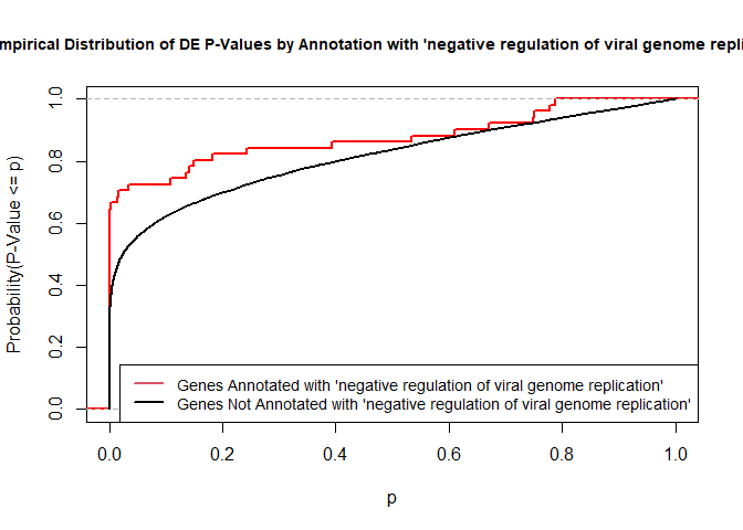
versus the probability distributions of p-values that are and that are not annotated with the term GO:0045071 “negative regulation of viral genome replication” (54 genes) p-value 3.3x10⁻⁹.
rna.pp.terms <- genesInTerm(GOdata)[["GO:0045071"]] # get genes associated with term
p.values.in <- geneList[names(geneList) %in% rna.pp.terms]
p.values.out <- geneList[!(names(geneList) %in% rna.pp.terms)]
plot.ecdf(p.values.in, verticals = T, do.points = F, col = "red", lwd = 2, xlim = c(0,1),
          main = "Empirical Distribution of DE P-Values by Annotation with 'negative regulation of viral genome replication'",
          cex.main = 0.9, xlab = "p", ylab = "Probability(P-Value <= p)")
ecdf.out <- ecdf(p.values.out)
xx <- unique(sort(c(seq(0, 1, length = 201), knots(ecdf.out))))
lines(xx, ecdf.out(xx), col = "black", lwd = 2)
legend("bottomright", legend = c("Genes Annotated with 'negative regulation of viral genome replication'", "Genes Not Annotated with 'negative regulation of viral genome replication'"), lwd = 2, col = 2:1, cex = 0.9)
We can use the function showSigOfNodes to plot the GO graph for the 2 most significant terms and their parents, color coded by enrichment p-value (red is most significant):
par(cex = 0.3)
showSigOfNodes(GOdata, score(resultKS), firstSigNodes = 2, useInfo = "def", .NO.CHAR = 40)
## Loading required package: Rgraphviz
## Loading required package: grid
##
## Attaching package: 'grid'
## The following object is masked from 'package:topGO':
##
##     depth
##
## Attaching package: 'Rgraphviz'
## The following objects are masked from 'package:IRanges':
##
##     from, to
## The following objects are masked from 'package:S4Vectors':
##
##     from, to
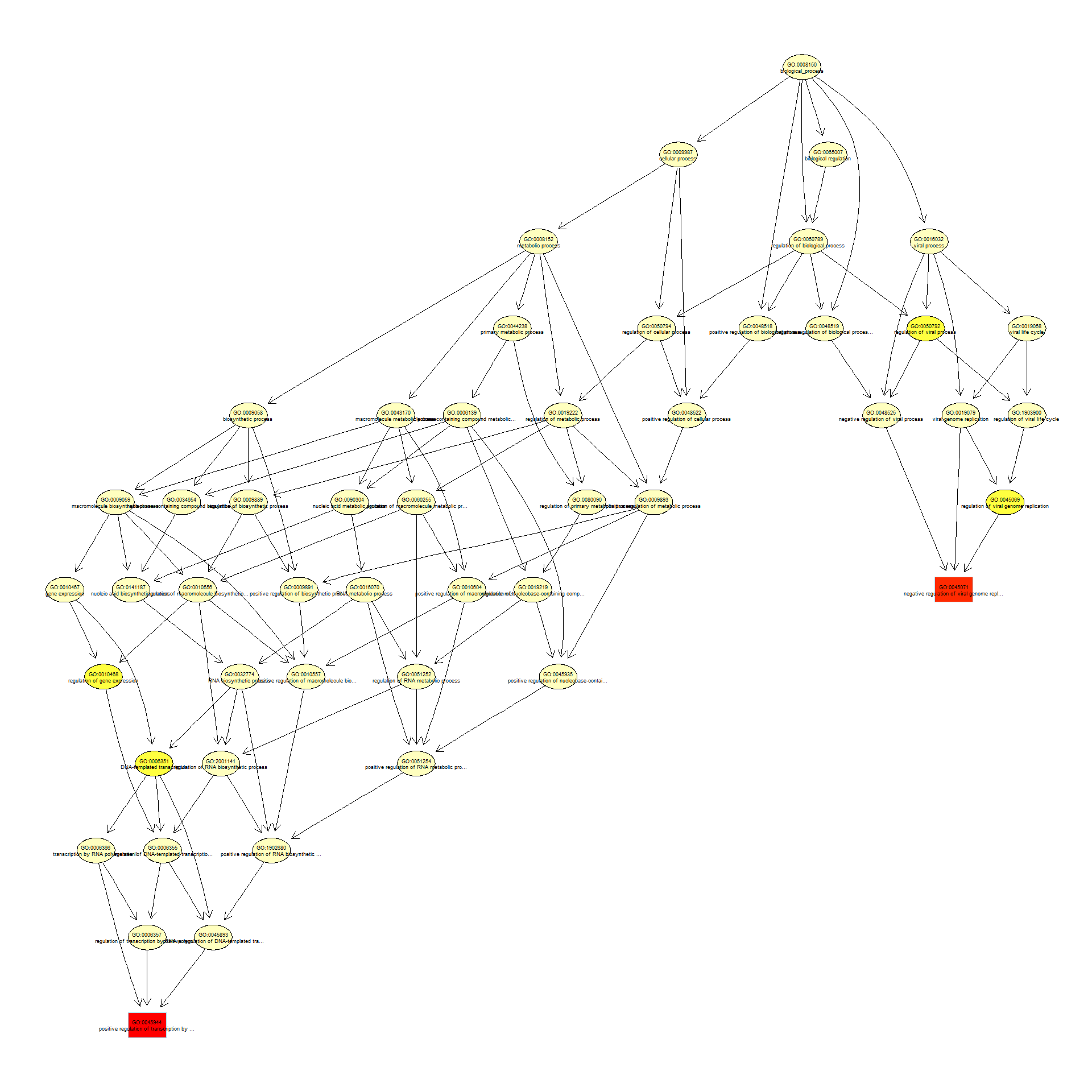
## $dag
## A graphNEL graph with directed edges
## Number of Nodes = 50
## Number of Edges = 106
##
## $complete.dag
## [1] "A graph with 50 nodes."
par(cex = 1)
3. topGO Example Using Fisher’s Exact Test
Next, we use Fisher’s exact test to test for GO enrichment among significantly DE genes.
Create topGOdata object:
geneList <- DE.nodupENTREZ$adj.P.Val
names(geneList) <- DE.nodupENTREZ$ENTREZID

# Create topGOData object
GOdata <- new("topGOdata",
	ontology = "BP",
	allGenes = geneList,
	geneSelectionFun = function(x) (x < 0.05),
	annot = annFUN.org , mapping = "org.Mm.eg.db")
##
## Building most specific GOs .....
## ( 10608 GO terms found. )
##
## Build GO DAG topology ..........
## ( 13703 GO terms and 30140 relations. )
##
## Annotating nodes ...............
## ( 10477 genes annotated to the GO terms. )
Run Fisher’s Exact Test:
resultFisher <- runTest(GOdata, algorithm = "elim", statistic = "fisher")
##
## 			 -- Elim Algorithm --
##
## 		 the algorithm is scoring 12186 nontrivial nodes
## 		 parameters:
## 			 test statistic: fisher
## 			 cutOff: 0.01
##
## 	 Level 19:	2 nodes to be scored	(0 eliminated genes)
##
## 	 Level 18:	21 nodes to be scored	(0 eliminated genes)
##
## 	 Level 17:	45 nodes to be scored	(8 eliminated genes)
##
## 	 Level 16:	82 nodes to be scored	(8 eliminated genes)
##
## 	 Level 15:	111 nodes to be scored	(26 eliminated genes)
##
## 	 Level 14:	205 nodes to be scored	(61 eliminated genes)
##
## 	 Level 13:	464 nodes to be scored	(357 eliminated genes)
##
## 	 Level 12:	860 nodes to be scored	(479 eliminated genes)
##
## 	 Level 11:	1328 nodes to be scored	(1920 eliminated genes)
##
## 	 Level 10:	1610 nodes to be scored	(2302 eliminated genes)
##
## 	 Level 9:	1784 nodes to be scored	(2944 eliminated genes)
##
## 	 Level 8:	1732 nodes to be scored	(3741 eliminated genes)
##
## 	 Level 7:	1518 nodes to be scored	(4483 eliminated genes)
##
## 	 Level 6:	1215 nodes to be scored	(5243 eliminated genes)
##
## 	 Level 5:	740 nodes to be scored	(6306 eliminated genes)
##
## 	 Level 4:	354 nodes to be scored	(6861 eliminated genes)
##
## 	 Level 3:	97 nodes to be scored	(7022 eliminated genes)
##
## 	 Level 2:	17 nodes to be scored	(7107 eliminated genes)
##
## 	 Level 1:	1 nodes to be scored	(7142 eliminated genes)
tab <- GenTable(GOdata, raw.p.value = resultFisher, topNodes = length(resultFisher@score),
				numChar = 120)
head(tab)
##        GO.ID                                                       Term
## 1 GO:0001525                                               angiogenesis
## 2 GO:0007204 positive regulation of cytosolic calcium ion concentration
## 3 GO:0007165                                        signal transduction
## 4 GO:0032731       positive regulation of interleukin-1 beta production
## 5 GO:0045944  positive regulation of transcription by RNA polymerase II
## 6 GO:0032760    positive regulation of tumor necrosis factor production
##   Annotated Significant Expected raw.p.value
## 1       324         225   163.62     1.6e-07
## 2        77          60    38.89     6.3e-07
## 3      3123        1817  1577.15     1.1e-06
## 4        54          44    27.27     2.3e-06
## 5       800         464   404.01     5.8e-06
## 6        97          70    48.99     1.1e-05
- Annotated: number of genes (in our gene list) that are annotated with the term
- Significant: Number of significantly DE genes annotated with that term (i.e. genes where geneList = 1)
- Expected: Under random chance, number of genes that would be expected to be significantly DE and annotated with that term
- raw.p.value: P-value from Fisher’s Exact Test, testing for association between significance and pathway membership.
Fisher’s Exact Test is applied to the table:
| Significance/Annotation | Annotated With GO Term | Not Annotated With GO Term |
|---|---|---|
| Significantly DE | n1 | n3 |
| Not Significantly DE | n2 | n4 |
and compares the probability of the observed table, conditional on the row and column sums, to what would be expected under random chance.
Advantages over KS (or Wilcoxon) Tests:
-
Ease of interpretation
-
Can be applied when you just have a gene list without associated p-values, etc.
Disadvantages:
- Relies on significant/non-significant dichotomy (an interesting gene could have an adjusted p-value of 0.051 and be counted as non-significant)
- Less powerful
- May be less useful if there are very few (or a large number of) significant genes
Quiz 1
KEGG Pathway Enrichment Testing With clusterProfiler
KEGG, the Kyoto Encyclopedia of Genes and Genomes (https://www.genome.jp/kegg/), provides assignment of genes for many organisms into pathways.
We will conduct KEGG enrichment testing using the Bioconductor package clusterProfiler. clusterProfiler implements an algorithm very similar to that used by GSEA.
Cluster profiler can do much more than KEGG enrichment, check out the clusterProfiler book.
We will base our KEGG enrichment analysis on the t statistics from differential expression, which allows for directional testing.
geneList.KEGG <- DE.nodupENTREZ$t
geneList.KEGG <- sort(geneList.KEGG, decreasing = TRUE)
names(geneList.KEGG) <- DE.nodupENTREZ$ENTREZID
head(geneList.KEGG)
##    67241    68891    12772    70686   219140    94212
## 40.72759 39.08710 32.14372 31.47893 29.40610 29.38849
set.seed(99)
KEGG.results <- gseKEGG(gene = geneList.KEGG, organism = "mmu", pvalueCutoff = 1)
## Reading KEGG annotation online: "https://rest.kegg.jp/link/mmu/pathway"...
## Reading KEGG annotation online: "https://rest.kegg.jp/list/pathway/mmu"...
## using 'fgsea' for GSEA analysis, please cite Korotkevich et al (2019).
## preparing geneSet collections...
## GSEA analysis...
## leading edge analysis...
## done...
KEGG.results <- setReadable(KEGG.results, OrgDb = "org.Mm.eg.db", keyType = "ENTREZID")
outdat <- as.data.frame(KEGG.results)
head(outdat)
##                ID                                     Description setSize
## mmu04514 mmu04514                         Cell adhesion molecules      74
## mmu04015 mmu04015                          Rap1 signaling pathway     125
## mmu04380 mmu04380                      Osteoclast differentiation     113
## mmu04662 mmu04662               B cell receptor signaling pathway      75
## mmu05167 mmu05167 Kaposi sarcoma-associated herpesvirus infection     151
## mmu04062 mmu04062                     Chemokine signaling pathway     122
##          enrichmentScore      NES       pvalue     p.adjust       qvalue rank
## mmu04514       0.6190383 2.193009 6.147516e-08 1.151476e-05 7.123299e-06 1257
## mmu04015       0.5356389 2.056773 7.086005e-08 1.151476e-05 7.123299e-06 2197
## mmu04380       0.5459626 2.072437 1.551850e-07 1.681171e-05 1.040012e-05 2226
## mmu04662       0.5944450 2.111142 2.550558e-07 2.072328e-05 1.281991e-05 2203
## mmu05167       0.4875951 1.928343 5.961922e-07 3.875249e-05 2.397320e-05 1525
## mmu04062       0.5115253 1.961990 1.063325e-06 5.244683e-05 3.244484e-05 2197
##                            leading_edge
## mmu04514 tags=34%, list=12%, signal=30%
## mmu04015 tags=49%, list=20%, signal=39%
## mmu04380 tags=42%, list=20%, signal=34%
## mmu04662 tags=49%, list=20%, signal=40%
## mmu05167 tags=31%, list=14%, signal=27%
## mmu04062 tags=43%, list=20%, signal=35%
##                                                                                                                                                                                                                                                                                                                                                                 core_enrichment
## mmu04514                                                                                                                                                                                                                   Vcan/Spn/Cd274/Sell/Itgal/L1cam/Itgb1/Itgb2/Vsir/H2-Q6/Pecam1/Jaml/Pdcd1lg2/H2-K1/H2-Q7/H2-Q4/H2-D1/Siglec1/Itgav/H2-T24/Cd22/H2-Ob/Cadm3/Cdh1/Itgb7
## mmu04015 Plcb1/Sipa1l1/Tiam1/Met/Adcy7/Thbs1/Itgal/Itgb1/Itgb2/Calm1/Afdn/Rassf5/Raf1/Rap1b/Pdgfb/Gnaq/Vasp/Evl/Rasgrp2/Vegfc/Rras/Sipa1l3/Insr/P2ry1/Prkd2/Prkcb/Actg1/Fpr1/Rapgef5/Map2k1/Pik3cd/Pfn1/Hgf/Rap1a/Rapgef1/Apbb1ip/Csf1r/Rhoa/Cdh1/Rac1/Tln1/Adora2a/Fgfr1/Kras/Adcy4/Akt1/Lcp2/Crk/Itgb3/Mapk3/Pdgfrb/Ralb/Rgs14/Plcb3/Fyb1/Arap3/Akt3/Calml4/Pik3r2/Adcy9/Vav3
## mmu04380                                                                     Pparg/Lilra6/Lilra5/Fyn/Fcgr4/Stat2/Itpr1/Pira11/Tgfbr1/Acp5/Sirpd/Tyk2/Pirb/Ncf1/Map3k14/Mitf/Tgfbr2/Pira2/Nfkb1/Itpr3/Fcgr1/Map2k1/Pik3cd/Spi1/Socs3/Pira1/Trem2/Sqstm1/Csf1r/Pira6/Rac1/Fos/Ppp3r1/Nfatc1/Lilrb4b/Akt1/Nfkbia/Lcp2/Itgb3/Mapk3/Gab2/Sirpb1a/Chuk/Akt3/Tab2/Pik3r2/Fcgr2b/Ifngr1
## mmu04662                                                                                                                                       Lilra6/Lilra5/Pik3ap1/Nfatc3/Raf1/Cd81/Pira11/Pirb/Ptpn6/Cd79a/Pira2/Prkcb/Nfkb1/Cd22/Map2k1/Ifitm1/Pik3cd/Pira1/Cd19/Pira6/Rac1/Fos/Ppp3r1/Nfatc1/Kras/Lilrb4b/Akt1/Nfkbia/Blk/Mapk3/Nfkbie/Chuk/Akt3/Pik3r2/Inppl1/Vav3/Fcgr2b
## mmu05167                                                                                       C3/Pik3r6/Rcan1/Tcf7l2/Nfatc3/H2-Q6/Calm1/Gng2/Stat2/Raf1/Itpr1/Pdgfb/Tyk2/E2f2/H2-K1/H2-Q7/Rb1/Ccr1/Il6st/H2-Q4/H2-D1/Gngt2/Traf3/Hck/H2-T24/Nfkb1/Ikbke/Eif2ak2/Itpr3/Stat3/Map2k1/Pik3cd/Irf7/Casp8/Gnb1/Rac1/Fos/Ppp3r1/Jak2/Irf3/Nfatc1/Hif1a/Kras/Cdk6/Akt1/Nfkbia/Cd200r1
## mmu04062                                                           Ccr2/Plcb1/Tiam1/Pik3r6/Adcy7/Grk3/Ccl9/Ptk2b/Gng2/Stat2/Ccl6/Raf1/Rap1b/Gnaq/Cxcr4/Rasgrp2/Ccr1/Ncf1/Gngt2/Cxcl10/Prkcb/Hck/Nfkb1/Stat5b/Stat3/Map2k1/Pik3cd/Ccl2/Rap1a/Gnb1/Rhoa/Gsk3a/Rac1/Jak2/Bad/Kras/Adcy4/Akt1/Fgr/Nfkbia/Crk/Mapk3/Elmo1/Prkacb/Plcb3/Gng10/Chuk/Akt3/Grk2/Cx3cr1/Pik3r2/Adcy9/Vav3
Gene set enrichment analysis output includes the following columns:
-
setSize: Number of genes in pathway
-
enrichmentScore: GSEA enrichment score, a statistic reflecting the degree to which a pathway is overrepresented at the top or bottom of the gene list (the gene list here consists of the t-statistics from the DE test).
-
pvalue: Raw p-value from permutation test of enrichment score
-
p.adjust: Benjamini-Hochberg false discovery rate adjusted p-value
-
qvalue: Storey false discovery rate adjusted p-value
-
rank: Position in ranked list at which maximum enrichment score occurred
-
leading_edge: Statistics from leading edge analysis
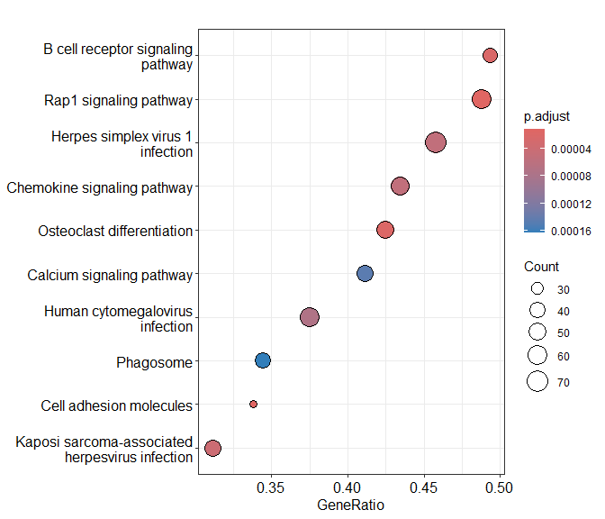
Dotplot of enrichment results
Gene.ratio = (count of core enrichment genes)/(count of pathway genes)
Core enrichment genes = subset of genes that contribute most to the enrichment result (“leading edge subset”)
dotplot(KEGG.results)
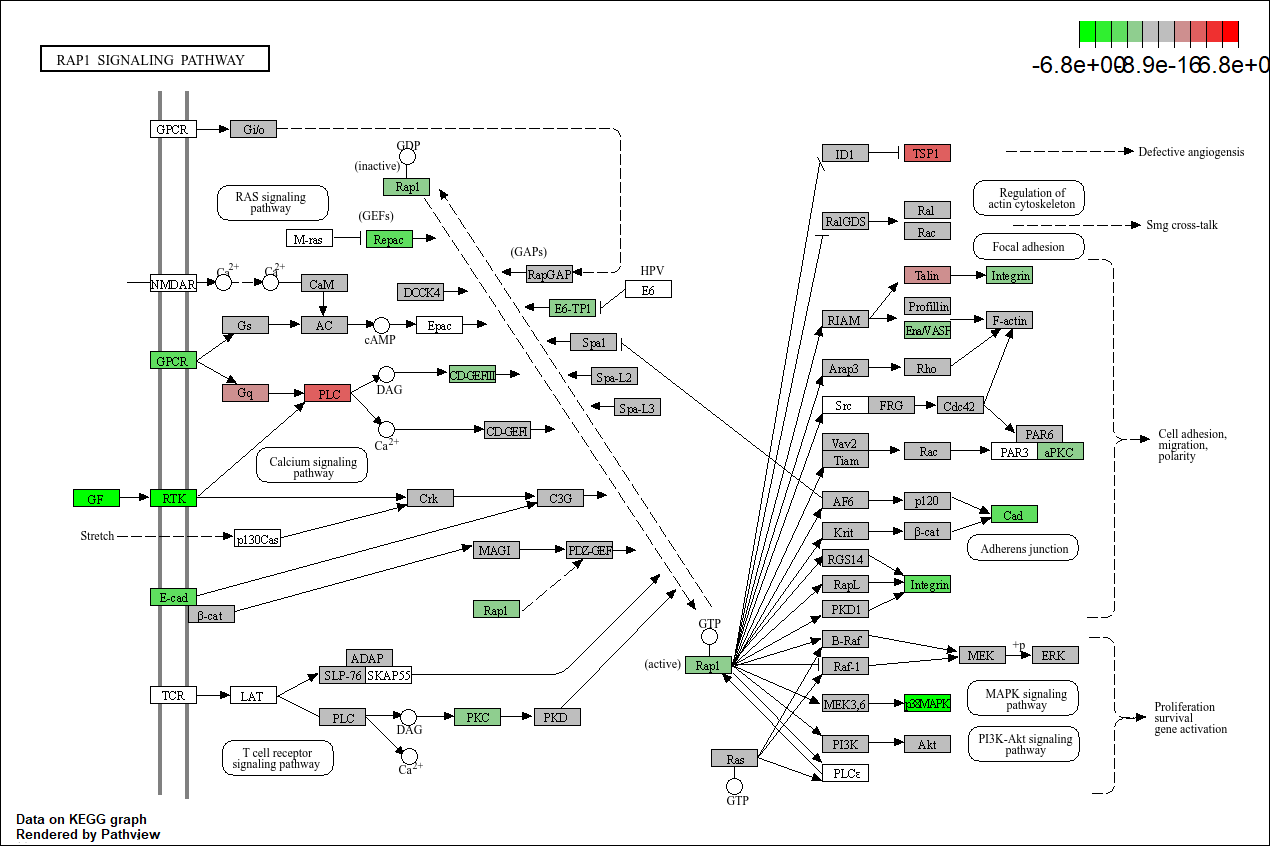
Pathview plot of log fold changes on KEGG diagram
foldChangeList <- DE$logFC
xx <- as.list(org.Mm.egENSEMBL2EG)
names(foldChangeList) <- xx[sapply(strsplit(DE$Gene,split="\\."),"[[", 1L)]
head(foldChangeList)
##     67241     68891     12772     70686    219140     94212
## -2.474865  4.558642  2.171072 -4.109923 -2.668725 -1.888581
mmu04015 <- pathview(gene.data  = foldChangeList,
                     pathway.id = "mmu04015",
                     species    = "mmu",
                     limit      = list(gene=max(abs(foldChangeList)), cpd=1))
## 'select()' returned 1:1 mapping between keys and columns
## Info: Working in directory C:/Users/bpdurbin/OneDrive - University of California, Davis/work_stuff/2025-June-RNA-Seq-Analysis/data_analysis
## Info: Writing image file mmu04015.pathview.png
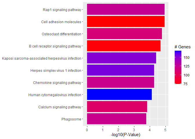
Barplot of p-values for top pathways
A barplot of -log10(p-value) for the top pathways/terms can be used for any type of enrichment analysis.
plotdat <- outdat[1:10,]
plotdat$nice.name <- gsub(" - Mus musculus (house mouse)", "", plotdat$Description, fixed = TRUE)

ggplot(plotdat, aes(x = -log10(p.adjust), y = reorder(nice.name, -log10(p.adjust)), fill = setSize)) + geom_bar(stat = "identity") + labs(x = "-log10(P-Value)", y = NULL, fill = "# Genes") + scale_fill_gradient(low = "red", high = "blue")
Quiz 2
sessionInfo()
## R version 4.5.0 (2025-04-11 ucrt)
## Platform: x86_64-w64-mingw32/x64
## Running under: Windows 11 x64 (build 26100)
##
## Matrix products: default
##   LAPACK version 3.12.1
##
## locale:
## [1] LC_COLLATE=English_United States.utf8
## [2] LC_CTYPE=English_United States.utf8
## [3] LC_MONETARY=English_United States.utf8
## [4] LC_NUMERIC=C
## [5] LC_TIME=English_United States.utf8
##
## time zone: America/Los_Angeles
## tzcode source: internal
##
## attached base packages:
## [1] grid      stats4    stats     graphics  grDevices utils     datasets
## [8] methods   base
##
## other attached packages:
##  [1] Rgraphviz_2.52.0       dplyr_1.1.4            ggplot2_3.5.2
##  [4] enrichplot_1.28.2      pathview_1.48.0        clusterProfiler_4.16.0
##  [7] org.Mm.eg.db_3.21.0    topGO_2.59.0           SparseM_1.84-2
## [10] GO.db_3.21.0           AnnotationDbi_1.70.0   IRanges_2.42.0
## [13] S4Vectors_0.46.0       Biobase_2.68.0         graph_1.86.0
## [16] BiocGenerics_0.54.0    generics_0.1.4
##
## loaded via a namespace (and not attached):
##  [1] bitops_1.0-9            DBI_1.2.3               gson_0.1.0
##  [4] rlang_1.1.6             magrittr_2.0.3          DOSE_4.2.0
##  [7] matrixStats_1.5.0       compiler_4.5.0          RSQLite_2.3.11
## [10] png_0.1-8               vctrs_0.6.5             reshape2_1.4.4
## [13] stringr_1.5.1           pkgconfig_2.0.3         crayon_1.5.3
## [16] fastmap_1.2.0           XVector_0.48.0          labeling_0.4.3
## [19] rmarkdown_2.29          KEGGgraph_1.68.0        UCSC.utils_1.4.0
## [22] purrr_1.0.4             bit_4.6.0               xfun_0.52
## [25] cachem_1.1.0            aplot_0.2.5             GenomeInfoDb_1.44.0
## [28] jsonlite_2.0.0          blob_1.2.4              BiocParallel_1.42.0
## [31] parallel_4.5.0          R6_2.6.1                bslib_0.9.0
## [34] stringi_1.8.7           RColorBrewer_1.1-3      jquerylib_0.1.4
## [37] GOSemSim_2.34.0         Rcpp_1.0.14             knitr_1.50
## [40] snow_0.4-4              ggtangle_0.0.6          R.utils_2.13.0
## [43] Matrix_1.7-3            splines_4.5.0           igraph_2.1.4
## [46] tidyselect_1.2.1        qvalue_2.40.0           yaml_2.3.10
## [49] codetools_0.2-20        lattice_0.22-6          tibble_3.2.1
## [52] plyr_1.8.9              withr_3.0.2             treeio_1.32.0
## [55] KEGGREST_1.48.0         evaluate_1.0.3          gridGraphics_0.5-1
## [58] Biostrings_2.76.0       pillar_1.10.2           ggtree_3.16.0
## [61] ggfun_0.1.8             RCurl_1.98-1.17         scales_1.4.0
## [64] tidytree_0.4.6          glue_1.8.0              lazyeval_0.2.2
## [67] tools_4.5.0             data.table_1.17.4       fgsea_1.34.0
## [70] XML_3.99-0.18           fs_1.6.6                fastmatch_1.1-6
## [73] cowplot_1.1.3           tidyr_1.3.1             ape_5.8-1
## [76] nlme_3.1-168            GenomeInfoDbData_1.2.14 patchwork_1.3.0
## [79] cli_3.6.5               gtable_0.3.6            R.methodsS3_1.8.2
## [82] yulab.utils_0.2.0       sass_0.4.10             digest_0.6.37
## [85] ggrepel_0.9.6           ggplotify_0.1.2         org.Hs.eg.db_3.21.0
## [88] farver_2.1.2            memoise_2.0.1           htmltools_0.5.8.1
## [91] R.oo_1.27.1             lifecycle_1.0.4         httr_1.4.7
## [94] bit64_4.6.0-1