Home
Introduction and Lectures
Intro to the Workshop and Core
Schedule
Talk by Diana Burkhat-Waco from 10x Genomics
What is Bioinformatics/Genomics?
Experimental Design and Cost Estimation
Support
Zoom
Slack
Cheat Sheets
Software and Links
Scripts
Prerequisites
CLI
R
Data Reduction
Project setup
Generating Expression Matrix
scRNAseq Analysis
Prepare scRNAseq Analysis
scRNAseq Analysis - PART1
scRNAseq Analysis - PART2
scRNAseq Analysis - PART3
scRNAseq Analysis - PART4
scRNAseq Analysis - PART5
scRNAseq Analysis - PART6
Shiny App Data Explore
Shiny App on AWS (extra)
ETC
Closing thoughts
Github page
Biocore website

Last Updated: March 23 2021, 5pm

Part 1: Loading data from CellRanger into R

Our first Markdown document concentrates on getting data into R and setting up our initial object.

Single Cell Analysis with Seurat and some custom code!

Seurat (now Version 4) is a popular R package that is designed for QC, analysis, and exploration of single cell data. Seurat aims to enable users to identify and interpret sources of heterogeneity from single cell transcriptomic measurements, and to integrate diverse types of single cell data. Further, the authors provide several tutorials, on their website.

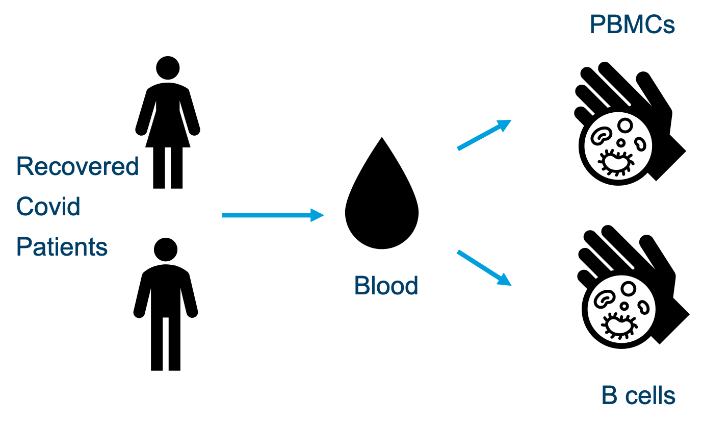
The intro2singlecell_March2021.zip file contains the single cell matrix files and HDF5 files for four Covid positive PBMc samples. These are PBMC human cells ran on the 10X genomics platform (5’ gene expression kit V2 with b-cell VDJ) for single cell RNA sequencing, sequenced with UC Davis in Nov and Dec of 2020 on a NovaSeq 6000. The experiment for the workshop contains 4 samples, each merged from 2 original samples and “normal” PBMC data from 10X Genomics.

Covid

The four samples are,

PBMC2 - Performed in Nov
PBMC3 - Performed in Nov
T021 - Performed in Dec
T022 - Performed in Dec

Also in the directory is the 10X “normal” PBMC dataset

We start each markdown document with loading needed libraries for R

# must have Seurat
library(Seurat)
library(kableExtra)
library(ggplot2)

Setup the experiment folder and data info

experiment_name = "Covid Example"
dataset_loc <- "./intro2singlecell_March2021"
ids <- c("PBMC2", "PBMC3", "T021PBMC", "T022PBMC")

Read in the cellranger sample metrics csv files

d10x.metrics <- lapply(ids, function(i){
  # remove _Counts is if names don't include them
  metrics <- read.csv(file.path(dataset_loc,paste0(i,"_Counts/outs"),"metrics_summary.csv"), colClasses = "character")
})
experiment.metrics <- do.call("rbind", d10x.metrics)
rownames(experiment.metrics) <- ids

sequencing_metrics <- data.frame(t(experiment.metrics[,c(4:17,1,18,2,3,19,20)]))

row.names(sequencing_metrics) <- gsub("\\."," ", rownames(sequencing_metrics))

And lets generate a pretty table

sequencing_metrics %>%
  kable(caption = 'Cell Ranger Results') %>%
  pack_rows("Sequencing Characteristics", 1, 7, label_row_css = "background-color: #666; color: #fff;") %>%
  pack_rows("Mapping Characteristics", 8, 14, label_row_css = "background-color: #666; color: #fff;") %>%
  pack_rows("Cell Characteristics", 15, 20, label_row_css = "background-color: #666; color: #fff;") %>%
  kable_styling("striped")

Cell Ranger Results
	PBMC2	PBMC3	T021PBMC	T022PBMC
Sequencing Characteristics
Number of Reads	313,087,958	339,008,152	364,881,065	358,269,446
Valid Barcodes	85.1%	82.0%	91.5%	91.0%
Sequencing Saturation	78.8%	76.5%	85.2%	87.3%
Q30 Bases in Barcode	97.2%	97.1%	94.3%	94.4%
Q30 Bases in RNA Read	94.5%	94.5%	87.3%	87.4%
Q30 Bases in RNA Read 2	91.1%	91.1%	89.3%	88.7%
Q30 Bases in UMI	96.9%	96.9%	93.9%	94.0%
Mapping Characteristics
Reads Mapped to Genome	91.2%	91.3%	90.9%	90.0%
Reads Mapped Confidently to Genome	70.0%	69.4%	83.5%	82.9%
Reads Mapped Confidently to Intergenic Regions	5.8%	5.5%	4.1%	4.4%
Reads Mapped Confidently to Intronic Regions	8.9%	7.3%	6.6%	6.9%
Reads Mapped Confidently to Exonic Regions	55.3%	56.7%	72.9%	71.6%
Reads Mapped Confidently to Transcriptome	48.6%	48.2%	67.3%	65.6%
Reads Mapped Antisense to Gene	4.3%	6.5%	3.0%	3.4%
Cell Characteristics
Estimated Number of Cells	6,914	7,483	7,891	5,120
Fraction Reads in Cells	53.2%	89.5%	92.0%	92.6%
Mean Reads per Cell	45,283	45,304	46,240	69,975
Median Genes per Cell	840	1,385	1,506	1,739
Total Genes Detected	20,425	20,681	21,012	20,774
Median UMI Counts per Cell	1,506	3,384	3,912	4,736

Load the Cell Ranger Matrix Data and create the base Seurat object.

Cell Ranger provides a function cellranger aggr that will combine multiple samples into a single matrix file. However, when processing data in R this is unnecessary and we can quickly aggregate them in R.

Seurat provides a function Read10X and Read10X_h5 to read in 10X data folder. First we read in data from each individual sample folder.

Later, we initialize the Seurat object (CreateSeuratObject) with the raw (non-normalized data). Keep all cells with at least 200 detected genes. Also extracting sample names, calculating and adding in the metadata mitochondrial percentage of each cell. Adding in the metadata batchid and cell cycle. Finally, saving the raw Seurat object.

Load the Cell Ranger Matrix Data (hdf5 file) and create the base Seurat object.

d10x.data <- lapply(ids, function(i){
  d10x <- Read10X_h5(file.path(dataset_loc,paste0(i,"_Counts/outs"),"raw_feature_bc_matrix.h5"))
  colnames(d10x) <- paste(sapply(strsplit(colnames(d10x),split="-"),'[[',1L),i,sep="-")
  d10x
})
names(d10x.data) <- ids

str(d10x.data)

List of 4 $ PBMC2 :Formal class 'dgCMatrix' [package "Matrix"] with 6 slots .. ..@ i : int [1:18215841] 84 565 796 915 943 975 1475 1832 2059 2061 ... .. ..@ p : int [1:507423] 0 206 207 208 209 432 437 437 439 441 ... .. ..@ Dim : int [1:2] 36601 507422 .. ..@ Dimnames:List of 2 .. .. ..$ : chr [1:36601] "MIR1302-2HG" "FAM138A" "OR4F5" "AL627309.1" ... .. .. ..$ : chr [1:507422] "AAACCTGAGAAACCAT-PBMC2" "AAACCTGAGAAACCGC-PBMC2" "AAACCTGAGAACAACT-PBMC2" "AAACCTGAGAACAATC-PBMC2" ... .. ..@ x : num [1:18215841] 1 1 1 1 1 1 1 1 1 1 ... .. ..@ factors : list() $ PBMC3 :Formal class 'dgCMatrix' [package "Matrix"] with 6 slots .. ..@ i : int [1:14111379] 1832 34974 593 847 1944 2061 4261 8706 11613 12196 ... .. ..@ p : int [1:522341] 0 2 31 32 34 34 34 34 34 34 ... .. ..@ Dim : int [1:2] 36601 522340 .. ..@ Dimnames:List of 2 .. .. ..$ : chr [1:36601] "MIR1302-2HG" "FAM138A" "OR4F5" "AL627309.1" ... .. .. ..$ : chr [1:522340] "AAACCTGAGAAACCAT-PBMC3" "AAACCTGAGAAACCTA-PBMC3" "AAACCTGAGAAACGAG-PBMC3" "AAACCTGAGAAACGCC-PBMC3" ... .. ..@ x : num [1:14111379] 1 1 1 1 1 1 1 1 1 1 ... .. ..@ factors : list() $ T021PBMC:Formal class 'dgCMatrix' [package "Matrix"] with 6 slots .. ..@ i : int [1:14523505] 35378 29289 2314 21806 25903 10801 18939 28506 10468 33707 ... .. ..@ p : int [1:464418] 0 1 2 2 4 5 8 9 11 11 ... .. ..@ Dim : int [1:2] 36601 464417 .. ..@ Dimnames:List of 2 .. .. ..$ : chr [1:36601] "MIR1302-2HG" "FAM138A" "OR4F5" "AL627309.1" ... .. .. ..$ : chr [1:464417] "AAACCTGAGAAACCGC-T021PBMC" "AAACCTGAGAAAGTGG-T021PBMC" "AAACCTGAGAACAACT-T021PBMC" "AAACCTGAGAACAATC-T021PBMC" ... .. ..@ x : num [1:14523505] 1 1 1 1 1 2 1 1 1 1 ... .. ..@ factors : list() $ T022PBMC:Formal class 'dgCMatrix' [package "Matrix"] with 6 slots .. ..@ i : int [1:11234467] 53 610 2542 4334 4393 4421 5765 6163 7502 8756 ... .. ..@ p : int [1:438469] 0 0 0 43 46 46 68 99 100 105 ... .. ..@ Dim : int [1:2] 36601 438468 .. ..@ Dimnames:List of 2 .. .. ..$ : chr [1:36601] "MIR1302-2HG" "FAM138A" "OR4F5" "AL627309.1" ... .. .. ..$ : chr [1:438468] "AAACCTGAGAAACCTA-T022PBMC" "AAACCTGAGAAACGAG-T022PBMC" "AAACCTGAGAAACGCC-T022PBMC" "AAACCTGAGAAAGTGG-T022PBMC" ... .. ..@ x : num [1:11234467] 1 1 1 1 4 2 1 1 1 1 ... .. ..@ factors : list()

If you don’t have the needed hdf5 libraries you can read in the matrix files like such

d10x.data <- sapply(ids, function(i){
  d10x <- Read10X(file.path(dataset_loc,paste0(i,"_Counts/outs"),"raw_feature_bc_matrix"))
  colnames(d10x) <- paste(sapply(strsplit(colnames(d10x),split="-"),'[[',1L),i,sep="-")
  d10x
})
names(d10x.data) <- ids

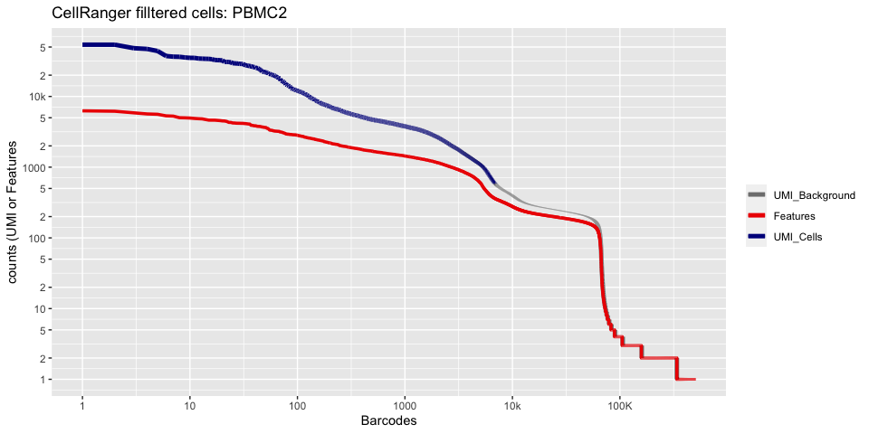
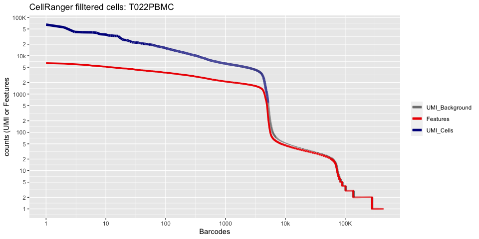
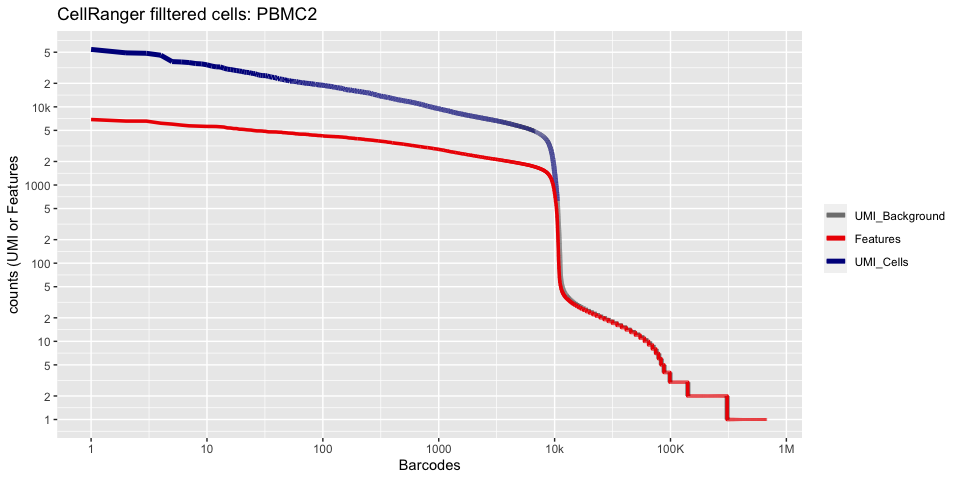
Lets recreate the pretty cellranger html plot

cr_filtered_cells <- as.numeric(gsub(",","",as.character(unlist(sequencing_metrics["Estimated Number of Cells",]))))

plot_cellranger_cells <- function(ind){
  xbreaks = c(1,1e1,1e2,1e3,1e4,1e5,1e6)
  xlabels = c("1","10","100","1000","10k","100K","1M")
  ybreaks = c(1,2,5,10,20,50,100,200,500,1000,2000,5000,10000,20000,50000,100000,200000,500000,1000000)
  ylabels = c("1","2","5","10","2","5","100","2","5","1000","2","5","10k","2","5","100K","2","5","1M")

  pl1 <- data.frame(index=seq.int(1,ncol(d10x.data[[ind]])), nCount_RNA = sort(Matrix:::colSums(d10x.data[[ind]])+1,decreasing=T), nFeature_RNA = sort(Matrix:::colSums(d10x.data[[ind]]>0)+1,decreasing=T)) %>% ggplot() + 
    scale_color_manual(values=c("grey50","red2","blue4"), labels=c("UMI_Background", "Features", "UMI_Cells"), name=NULL) +
    ggtitle(paste("CellRanger filltered cells:",ids[ind],sep=" ")) + xlab("Barcodes") + ylab("counts (UMI or Features") + 
    scale_x_continuous(trans = 'log2', breaks=xbreaks, labels = xlabels) + 
    scale_y_continuous(trans = 'log2', breaks=ybreaks, labels = ylabels) +
    geom_line(aes(x=index, y=nCount_RNA, color=index<=cr_filtered_cells[ind] , group=1), size=1.75) +
    geom_line(aes(x=index, y=nFeature_RNA, color="Features", group=1), size=1.25)

  return(pl1)
}

plot_cellranger_cells(1)

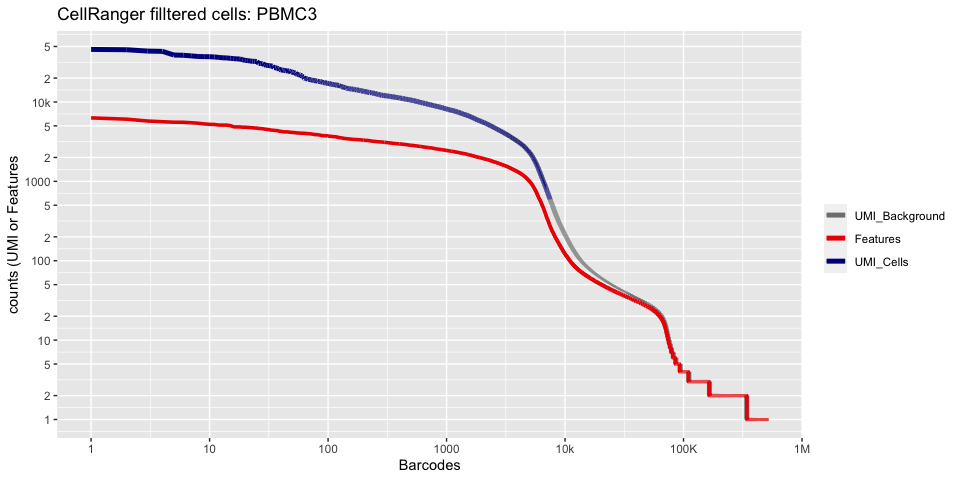
plot_cellranger_cells(2)

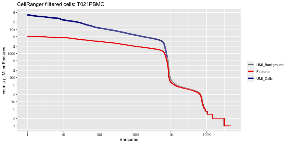
plot_cellranger_cells(3)

plot_cellranger_cells(4)

Create the Seurat object

filter criteria: remove genes that do not occur in a minimum of 0 cells and remove cells that don’t have a minimum of 200 features

experiment.data <- do.call("cbind", d10x.data)

experiment.aggregate <- CreateSeuratObject(
  experiment.data,
  project = experiment_name,
  min.cells = 0,
  min.features = 300,
  names.field = 2,
  names.delim = "\\-")

experiment.aggregate

An object of class Seurat 36601 features across 29696 samples within 1 assay Active assay: RNA (36601 features, 0 variable features)

str(experiment.aggregate)

Formal class 'Seurat' [package "SeuratObject"] with 13 slots ..@ assays :List of 1 .. ..$ RNA:Formal class 'Assay' [package "SeuratObject"] with 8 slots .. .. .. ..@ counts :Formal class 'dgCMatrix' [package "Matrix"] with 6 slots .. .. .. .. .. ..@ i : int [1:39483327] 62 78 438 524 631 647 829 920 975 1073 ... .. .. .. .. .. ..@ p : int [1:29697] 0 335 758 2331 3315 4444 4760 5983 7391 8653 ... .. .. .. .. .. ..@ Dim : int [1:2] 36601 29696 .. .. .. .. .. ..@ Dimnames:List of 2 .. .. .. .. .. .. ..$ : chr [1:36601] "MIR1302-2HG" "FAM138A" "OR4F5" "AL627309.1" ... .. .. .. .. .. .. ..$ : chr [1:29696] "AAACCTGAGCTAGTGG-PBMC2" "AAACCTGAGGCCCTTG-PBMC2" "AAACCTGAGGTGTGGT-PBMC2" "AAACCTGAGTCATGCT-PBMC2" ... .. .. .. .. .. ..@ x : num [1:39483327] 1 1 1 1 1 1 1 1 1 1 ... .. .. .. .. .. ..@ factors : list() .. .. .. ..@ data :Formal class 'dgCMatrix' [package "Matrix"] with 6 slots .. .. .. .. .. ..@ i : int [1:39483327] 62 78 438 524 631 647 829 920 975 1073 ... .. .. .. .. .. ..@ p : int [1:29697] 0 335 758 2331 3315 4444 4760 5983 7391 8653 ... .. .. .. .. .. ..@ Dim : int [1:2] 36601 29696 .. .. .. .. .. ..@ Dimnames:List of 2 .. .. .. .. .. .. ..$ : chr [1:36601] "MIR1302-2HG" "FAM138A" "OR4F5" "AL627309.1" ... .. .. .. .. .. .. ..$ : chr [1:29696] "AAACCTGAGCTAGTGG-PBMC2" "AAACCTGAGGCCCTTG-PBMC2" "AAACCTGAGGTGTGGT-PBMC2" "AAACCTGAGTCATGCT-PBMC2" ... .. .. .. .. .. ..@ x : num [1:39483327] 1 1 1 1 1 1 1 1 1 1 ... .. .. .. .. .. ..@ factors : list() .. .. .. ..@ scale.data : num[0 , 0 ] .. .. .. ..@ key : chr "rna_" .. .. .. ..@ assay.orig : NULL .. .. .. ..@ var.features : logi(0) .. .. .. ..@ meta.features:'data.frame': 36601 obs. of 0 variables .. .. .. ..@ misc : list() ..@ meta.data :'data.frame': 29696 obs. of 3 variables: .. ..$ orig.ident : Factor w/ 4 levels "PBMC2","PBMC3",..: 1 1 1 1 1 1 1 1 1 1 ... .. ..$ nCount_RNA : num [1:29696] 453 596 3606 1510 1856 ... .. ..$ nFeature_RNA: int [1:29696] 335 423 1573 984 1129 316 1223 1408 1262 872 ... ..@ active.assay: chr "RNA" ..@ active.ident: Factor w/ 4 levels "PBMC2","PBMC3",..: 1 1 1 1 1 1 1 1 1 1 ... .. ..- attr(*, "names")= chr [1:29696] "AAACCTGAGCTAGTGG-PBMC2" "AAACCTGAGGCCCTTG-PBMC2" "AAACCTGAGGTGTGGT-PBMC2" "AAACCTGAGTCATGCT-PBMC2" ... ..@ graphs : list() ..@ neighbors : list() ..@ reductions : list() ..@ images : list() ..@ project.name: chr "Covid Example" ..@ misc : list() ..@ version :Classes 'package_version', 'numeric_version' hidden list of 1 .. ..$ : int [1:3] 4 0 0 ..@ commands : list() ..@ tools : list()

Load the Cell Ranger Matrix Data with multiple tables (hdf5 file only) and create the base Seurat object.

normals <- c("10x_NormalPBMC_multi")

d10x.metrics <- lapply(normals, function(i){
  # remove _Counts is my names don't include them
  metrics <- read.csv(file.path(dataset_loc,paste0(i,"/outs"),"metrics_summary.csv"), colClasses = "character")
  metrics <- metrics[metrics$Library.Type == "Gene Expression",]
  metrics.new <- metrics$Metric.Value
  names(metrics.new) <- metrics$Metric.Name
  metrics.new
})

normal.metrics <- do.call("rbind", d10x.metrics)
rownames(normal.metrics) <- normals


d10x.normal <- lapply(normals, function(i){
  d10x <- Read10X_h5(file.path(dataset_loc,paste0(i,"/outs"),"raw_feature_bc_matrix.h5"))
  colnames(d10x$`Gene Expression`) <- paste(sapply(strsplit(colnames(d10x$`Gene Expression`),split="-"),'[[',1L),i,sep="-")
  colnames(d10x$`Antibody Capture`) <- paste(sapply(strsplit(colnames(d10x$`Antibody Capture`),split="-"),'[[',1L),i,sep="-")
  d10x
})
names(d10x.normal) <- normals

str(d10x.normal)

List of 1 $ 10x_NormalPBMC_multi:List of 2 ..$ Gene Expression :Formal class 'dgCMatrix' [package "Matrix"] with 6 slots .. .. ..@ i : int [1:21790216] 36386 31111 8220 31199 23735 32047 13246 26119 724 2093 ... .. .. ..@ p : int [1:702408] 0 1 1 2 4 4 4 4 4 4 ... .. .. ..@ Dim : int [1:2] 36601 702407 .. .. ..@ Dimnames:List of 2 .. .. .. ..$ : chr [1:36601] "MIR1302-2HG" "FAM138A" "OR4F5" "AL627309.1" ... .. .. .. ..$ : chr [1:702407] "AAACCTGAGAAACCAT-10x_NormalPBMC_multi" "AAACCTGAGAAACCGC-10x_NormalPBMC_multi" "AAACCTGAGAAACCTA-10x_NormalPBMC_multi" "AAACCTGAGAAACGAG-10x_NormalPBMC_multi" ... .. .. ..@ x : num [1:21790216] 1 1 1 1 1 2 1 1 1 1 ... .. .. ..@ factors : list() ..$ Antibody Capture:Formal class 'dgCMatrix' [package "Matrix"] with 6 slots .. .. ..@ i : int [1:3020346] 3 13 4 10 13 0 2 3 4 8 ... .. .. ..@ p : int [1:702408] 0 0 2 3 3 5 7 7 10 12 ... .. .. ..@ Dim : int [1:2] 19 702407 .. .. ..@ Dimnames:List of 2 .. .. .. ..$ : chr [1:19] "CD3_TotalC" "CD19_TotalC" "CD45RA_TotalC" "CD4_TotalC" ... .. .. .. ..$ : chr [1:702407] "AAACCTGAGAAACCAT-10x_NormalPBMC_multi" "AAACCTGAGAAACCGC-10x_NormalPBMC_multi" "AAACCTGAGAAACCTA-10x_NormalPBMC_multi" "AAACCTGAGAAACGAG-10x_NormalPBMC_multi" ... .. .. ..@ x : num [1:3020346] 1 1 1 1 1 1 1 1 1 1 ... .. .. ..@ factors : list()

How does d10x.data differ from d10x.normal?

cr_filtered_cells <- as.numeric(gsub(",","",as.character(unlist(normal.metrics[, "Estimated number of cells" ]))))

plot_cellranger_cells <- function(ind){
  xbreaks = c(1,1e1,1e2,1e3,1e4,1e5,1e6)
  xlabels = c("1","10","100","1000","10k","100K","1M")
  ybreaks = c(1,2,5,10,20,50,100,200,500,1000,2000,5000,10000,20000,50000,100000,200000,500000,1000000)
  ylabels = c("1","2","5","10","2","5","100","2","5","1000","2","5","10k","2","5","100K","2","5","1M")

  pl1 <- data.frame(index=seq.int(1,ncol(d10x.normal[[ind]][["Gene Expression"]])), nCount_RNA = sort(Matrix:::colSums(d10x.normal[[ind]][["Gene Expression"]])+1,decreasing=T), nFeature_RNA = sort(Matrix:::colSums(d10x.normal[[ind]][["Gene Expression"]]>0)+1,decreasing=T)) %>% ggplot() + 
    scale_color_manual(values=c("grey50","red2","blue4"), labels=c("UMI_Background", "Features", "UMI_Cells"), name=NULL) +
    ggtitle(paste("CellRanger filltered cells:",ids[ind],sep=" ")) + xlab("Barcodes") + ylab("counts (UMI or Features") + 
    scale_x_continuous(trans = 'log2', breaks=xbreaks, labels = xlabels) + 
    scale_y_continuous(trans = 'log2', breaks=ybreaks, labels = ylabels) +
    geom_line(aes(x=index, y=nCount_RNA, color=index<=cr_filtered_cells[ind] , group=1), size=1.75) +
    geom_line(aes(x=index, y=nFeature_RNA, color="Features", group=1), size=1.25)

  return(pl1)
}

plot_cellranger_cells(1)

Create the Seurat object

filter criteria: remove genes that do not occur in a minimum of 0 cells and remove cells that don’t have a minimum of 200 features

experiment.normal <- do.call("cbind", lapply(d10x.normal,"[[", "Gene Expression"))

experiment.aggregate.normal <- CreateSeuratObject(
  experiment.normal,
  project = "Normals",
  min.cells = 0,
  min.features = 300,
  names.field = 2,
  names.delim = "\\-")

experiment.aggregate

An object of class Seurat 36601 features across 29696 samples within 1 assay Active assay: RNA (36601 features, 0 variable features)

str(experiment.aggregate)

Lets create a metadata variable call batch, based on the sequencing run

Here we build a new metadata variable ‘batchid’ which can be used to specify treatment groups.

samplename = experiment.aggregate$orig.ident

batchid = rep("Batch1",length(samplename))
batchid[samplename %in% c("T021PBMC","T022PBMC")] = "Batch2"
names(batchid) = colnames(experiment.aggregate)

experiment.aggregate <- AddMetaData(
  object = experiment.aggregate,
  metadata = batchid,
  col.name = "batchid")

table(experiment.aggregate$batchid)

Batch1 Batch2 16298 13398

The percentage of reads that map to the mitochondrial genome

Low-quality / dying cells often exhibit extensive mitochondrial contamination.
We calculate mitochondrial QC metrics with the PercentageFeatureSet function, which calculates the percentage of counts originating from a set of features.
We use the set of all genes, in mouse these genes can be identified as those that begin with ‘mt’, in human data they begin with MT.

experiment.aggregate$percent.mito <- PercentageFeatureSet(experiment.aggregate, pattern = "^MT-")
summary(experiment.aggregate$percent.mito)

Min. 1st Qu. Median Mean 3rd Qu. Max. 0.000 1.672 2.637 4.098 4.493 66.956

Lets spend a little time getting to know the Seurat object.

The Seurat object is the center of each single cell analysis. It stores all information associated with the dataset, including data, annotations, analyses, etc. The R function slotNames can be used to view the slot names within an object.

slotNames(experiment.aggregate)

[1] "assays" "meta.data" "active.assay" "active.ident" "graphs" [6] "neighbors" "reductions" "images" "project.name" "misc" [11] "version" "commands" "tools"

head(experiment.aggregate[[]])

orig.ident nCount_RNA nFeature_RNA batchid percent.mito AAACCTGAGCTAGTGG-PBMC2 PBMC2 453 335 Batch1 1.3245033 AAACCTGAGGCCCTTG-PBMC2 PBMC2 596 423 Batch1 0.5033557 AAACCTGAGGTGTGGT-PBMC2 PBMC2 3606 1573 Batch1 3.1059346 AAACCTGAGTCATGCT-PBMC2 PBMC2 1510 984 Batch1 5.3642384 AAACCTGCAAACCCAT-PBMC2 PBMC2 1856 1129 Batch1 9.8060345 AAACCTGCAAAGAATC-PBMC2 PBMC2 646 316 Batch1 0.4643963

Question(s)

What slots are empty, what slots have data?
What columns are available in meta.data?
Look up the help documentation for subset?

Finally, save the original object and view the object.

Original dataset in Seurat class, with no filtering

save(experiment.aggregate,file="original_seurat_object.RData")
save(experiment.aggregate.normal,file="normal_seurat_object.RData")

Get the next Rmd file

download.file("https://raw.githubusercontent.com/ucdavis-bioinformatics-training/2021-March-Single-Cell-RNA-Seq-Analysis/master/data_analysis/scRNA_Workshop-PART2.Rmd", "scRNA_Workshop-PART2.Rmd")

Session Information

sessionInfo()

R version 4.0.3 (2020-10-10) Platform: x86_64-apple-darwin17.0 (64-bit) Running under: macOS Big Sur 10.16 Matrix products: default BLAS: /Library/Frameworks/R.framework/Versions/4.0/Resources/lib/libRblas.dylib LAPACK: /Library/Frameworks/R.framework/Versions/4.0/Resources/lib/libRlapack.dylib locale: [1] en_US.UTF-8/en_US.UTF-8/en_US.UTF-8/C/en_US.UTF-8/en_US.UTF-8 attached base packages: [1] stats graphics grDevices utils datasets methods base other attached packages: [1] ggplot2_3.3.3 kableExtra_1.3.4 SeuratObject_4.0.0 Seurat_4.0.1 loaded via a namespace (and not attached): [1] Rtsne_0.15 colorspace_2.0-0 deldir_0.2-10 [4] ellipsis_0.3.1 ggridges_0.5.3 rstudioapi_0.13 [7] spatstat.data_2.1-0 farver_2.1.0 leiden_0.3.7 [10] listenv_0.8.0 bit64_4.0.5 ggrepel_0.9.1 [13] fansi_0.4.2 xml2_1.3.2 codetools_0.2-18 [16] splines_4.0.3 knitr_1.31 polyclip_1.10-0 [19] jsonlite_1.7.2 ica_1.0-2 cluster_2.1.1 [22] png_0.1-7 uwot_0.1.10 shiny_1.6.0 [25] sctransform_0.3.2 spatstat.sparse_2.0-0 compiler_4.0.3 [28] httr_1.4.2 assertthat_0.2.1 Matrix_1.3-2 [31] fastmap_1.1.0 lazyeval_0.2.2 later_1.1.0.1 [34] htmltools_0.5.1.1 tools_4.0.3 igraph_1.2.6 [37] gtable_0.3.0 glue_1.4.2 RANN_2.6.1 [40] reshape2_1.4.4 dplyr_1.0.5 Rcpp_1.0.6 [43] scattermore_0.7 jquerylib_0.1.3 vctrs_0.3.6 [46] svglite_2.0.0 nlme_3.1-152 lmtest_0.9-38 [49] xfun_0.22 stringr_1.4.0 globals_0.14.0 [52] rvest_1.0.0 mime_0.10 miniUI_0.1.1.1 [55] lifecycle_1.0.0 irlba_2.3.3 goftest_1.2-2 [58] future_1.21.0 MASS_7.3-53.1 zoo_1.8-9 [61] scales_1.1.1 spatstat.core_2.0-0 promises_1.2.0.1 [64] spatstat.utils_2.1-0 parallel_4.0.3 RColorBrewer_1.1-2 [67] yaml_2.2.1 reticulate_1.18 pbapply_1.4-3 [70] gridExtra_2.3 sass_0.3.1 rpart_4.1-15 [73] stringi_1.5.3 highr_0.8 systemfonts_1.0.1 [76] rlang_0.4.10 pkgconfig_2.0.3 matrixStats_0.58.0 [79] evaluate_0.14 lattice_0.20-41 ROCR_1.0-11 [82] purrr_0.3.4 tensor_1.5 patchwork_1.1.1 [85] htmlwidgets_1.5.3 bit_4.0.4 cowplot_1.1.1 [88] tidyselect_1.1.0 parallelly_1.24.0 RcppAnnoy_0.0.18 [91] plyr_1.8.6 magrittr_2.0.1 R6_2.5.0 [94] generics_0.1.0 DBI_1.1.1 withr_2.4.1 [97] pillar_1.5.1 mgcv_1.8-34 fitdistrplus_1.1-3 [100] survival_3.2-10 abind_1.4-5 tibble_3.1.0 [103] future.apply_1.7.0 hdf5r_1.3.3 crayon_1.4.1 [106] KernSmooth_2.23-18 utf8_1.2.1 spatstat.geom_2.0-1 [109] plotly_4.9.3 rmarkdown_2.7 grid_4.0.3 [112] data.table_1.14.0 webshot_0.5.2 digest_0.6.27 [115] xtable_1.8-4 tidyr_1.1.3 httpuv_1.5.5 [118] munsell_0.5.0 viridisLite_0.3.0 bslib_0.2.4

☰ Menu

Single Cell RNA-Seq Analysis

Part 1: Loading data from CellRanger into R

Single Cell Analysis with Seurat and some custom code!

Setup the experiment folder and data info

Read in the cellranger sample metrics csv files

Load the Cell Ranger Matrix Data and create the base Seurat object.

Load the Cell Ranger Matrix Data (hdf5 file) and create the base Seurat object.

Create the Seurat object

Load the Cell Ranger Matrix Data with multiple tables (hdf5 file only) and create the base Seurat object.

Create the Seurat object

Lets create a metadata variable call batch, based on the sequencing run

The percentage of reads that map to the mitochondrial genome

Lets spend a little time getting to know the Seurat object.

Question(s)

Finally, save the original object and view the object.

Get the next Rmd file

Session Information