
Last Updated: March 24 2021, 11am
Part 3: Batch Correction Excercise
Load libraries
library(Seurat)
Load the Seurat object from the prior excercise, and create a batch effect
load(file="pre_sample_corrected.RData")
experiment.aggregate
An object of class Seurat
36601 features across 4000 samples within 1 assay
Active assay: RNA (36601 features, 3783 variable features)
experiment.test <- experiment.aggregate
VariableFeatures(experiment.test) <- rownames(experiment.test)
set.seed(12345)


samplename = experiment.aggregate$orig.ident
rand.cells <- sample(1:ncol(experiment.test), 2000,replace = F)
batchid = rep("Example_Batch1",length(samplename))
batchid[rand.cells] = "Example_Batch2"
names(batchid) = colnames(experiment.aggregate)

experiment.test <- AddMetaData(
  object = experiment.test,
  metadata = batchid,
  col.name = "example_batchid")

table(experiment.test$example_batchid)
Example_Batch1 Example_Batch2
2000 2000
mat <- as.matrix(GetAssayData(experiment.test, slot="data"))

rand.genes <- sample(VariableFeatures(experiment.test), 500,replace = F)

mat[rand.genes,experiment.test$example_batchid=="Example_Batch2"] <- mat[rand.genes,experiment.test$example_batchid=="Example_Batch2"] + 0.22
experiment.test = SetAssayData(experiment.test, slot="data", new.data= mat )
rm(mat)
Exploring Batch effects, none, Seurat [vars.to.regress]
First lets view the data without any corrections
PCA in prep for tSNE
ScaleData - Scales and centers genes in the dataset.
?ScaleData
experiment.test.noc <- ScaleData(object = experiment.test)
Run PCA
experiment.test.noc <- RunPCA(object = experiment.test.noc)
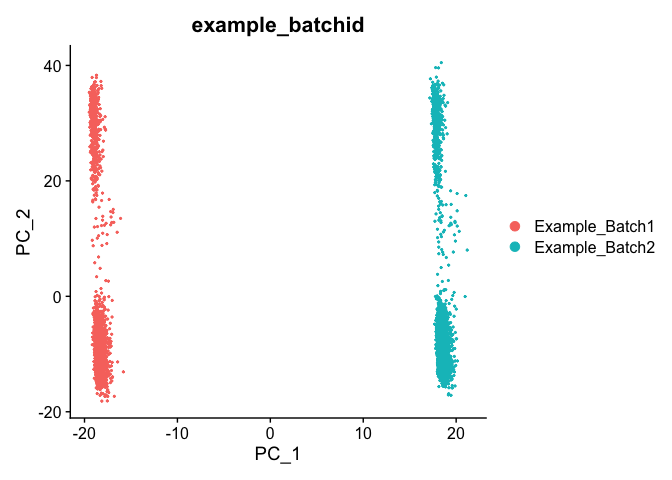
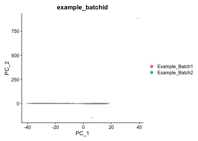
DimPlot(object = experiment.test.noc, group.by = "example_batchid", reduction = "pca")
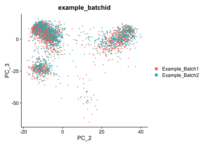
DimPlot(object = experiment.test.noc, group.by = "example_batchid", dims = c(2,3), reduction = "pca")
PCA Elbow plot to determine how many principal components to use in downstream analyses. Components after the “elbow” in the plot generally explain little additional variability in the data.
ElbowPlot(experiment.test.noc)
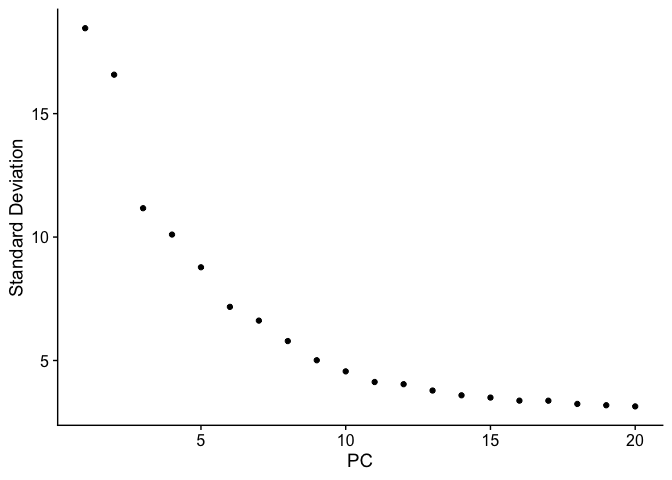
We use 10 components in downstream analyses. Using more components more closely approximates the full data set but increases run time.
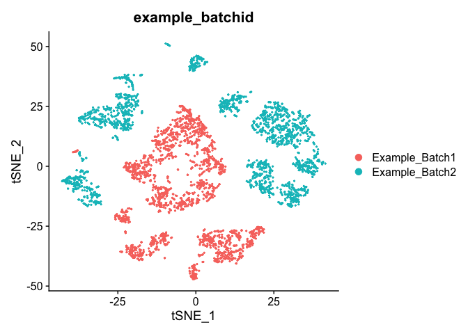
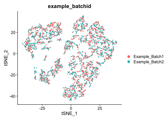
TSNE Plot
pcs.use <- 10
experiment.test.noc <- RunTSNE(object = experiment.test.noc, dims = 1:pcs.use)
DimPlot(object = experiment.test.noc,  group.by = "example_batchid")
Correct for sample to sample differences (seurat)
Use vars.to.regress to correct for the sample to sample differences and percent mitochondria
experiment.test.regress <- ScaleData(object = experiment.test,
                    vars.to.regress = c("example_batchid"), model.use = "linear")

experiment.test.regress <- RunPCA(object =experiment.test.regress,features=rownames(experiment.test.noc))

DimPlot(object = experiment.test.regress, group.by = "example_batchid", reduction = "pca")
Corrected TSNE Plot
experiment.test.regress <- RunTSNE(object = experiment.test.regress, dims.use = 1:50)
DimPlot(object = experiment.test.regress, group.by = "example_batchid", reduction = "tsne")
Question(s)
- Try a couple of PCA cutoffs (low and high) and compare the TSNE plots from the different methods. Do they look meaningfully different?
Excercise
Now go back to the original data without having been modified and see if a “batch effect” exists between the two actual batches
Get the next Rmd file
download.file("https://raw.githubusercontent.com/ucdavis-bioinformatics-training/2021-March-Single-Cell-RNA-Seq-Analysis/master/data_analysis/scRNA_Workshop-PART4.Rmd", "scRNA_Workshop-PART4.Rmd")
Session Information
sessionInfo()
R version 4.0.3 (2020-10-10)
Platform: x86_64-apple-darwin17.0 (64-bit)
Running under: macOS Big Sur 10.16
Matrix products: default
BLAS: /Library/Frameworks/R.framework/Versions/4.0/Resources/lib/libRblas.dylib
LAPACK: /Library/Frameworks/R.framework/Versions/4.0/Resources/lib/libRlapack.dylib
locale:
[1] en_US.UTF-8/en_US.UTF-8/en_US.UTF-8/C/en_US.UTF-8/en_US.UTF-8
attached base packages:
[1] stats graphics grDevices utils datasets methods base
other attached packages:
[1] SeuratObject_4.0.0 Seurat_4.0.1
loaded via a namespace (and not attached):
[1] Rtsne_0.15 colorspace_2.0-0 deldir_0.2-10
[4] ellipsis_0.3.1 ggridges_0.5.3 spatstat.data_2.1-0
[7] leiden_0.3.7 listenv_0.8.0 farver_2.1.0
[10] ggrepel_0.9.1 fansi_0.4.2 codetools_0.2-18
[13] splines_4.0.3 knitr_1.31 polyclip_1.10-0
[16] jsonlite_1.7.2 ica_1.0-2 cluster_2.1.1
[19] png_0.1-7 uwot_0.1.10 shiny_1.6.0
[22] sctransform_0.3.2 spatstat.sparse_2.0-0 compiler_4.0.3
[25] httr_1.4.2 assertthat_0.2.1 Matrix_1.3-2
[28] fastmap_1.1.0 lazyeval_0.2.2 later_1.1.0.1
[31] htmltools_0.5.1.1 tools_4.0.3 igraph_1.2.6
[34] gtable_0.3.0 glue_1.4.2 RANN_2.6.1
[37] reshape2_1.4.4 dplyr_1.0.5 Rcpp_1.0.6
[40] scattermore_0.7 jquerylib_0.1.3 vctrs_0.3.6
[43] nlme_3.1-152 lmtest_0.9-38 xfun_0.22
[46] stringr_1.4.0 globals_0.14.0 mime_0.10
[49] miniUI_0.1.1.1 lifecycle_1.0.0 irlba_2.3.3
[52] goftest_1.2-2 future_1.21.0 MASS_7.3-53.1
[55] zoo_1.8-9 scales_1.1.1 spatstat.core_2.0-0
[58] promises_1.2.0.1 spatstat.utils_2.1-0 parallel_4.0.3
[61] RColorBrewer_1.1-2 yaml_2.2.1 reticulate_1.18
[64] pbapply_1.4-3 gridExtra_2.3 ggplot2_3.3.3
[67] sass_0.3.1 rpart_4.1-15 stringi_1.5.3
[70] highr_0.8 rlang_0.4.10 pkgconfig_2.0.3
[73] matrixStats_0.58.0 evaluate_0.14 lattice_0.20-41
[76] ROCR_1.0-11 purrr_0.3.4 tensor_1.5
[79] patchwork_1.1.1 htmlwidgets_1.5.3 labeling_0.4.2
[82] cowplot_1.1.1 tidyselect_1.1.0 parallelly_1.24.0
[85] RcppAnnoy_0.0.18 plyr_1.8.6 magrittr_2.0.1
[88] R6_2.5.0 generics_0.1.0 DBI_1.1.1
[91] pillar_1.5.1 mgcv_1.8-34 fitdistrplus_1.1-3
[94] survival_3.2-10 abind_1.4-5 tibble_3.1.0
[97] future.apply_1.7.0 crayon_1.4.1 KernSmooth_2.23-18
[100] utf8_1.2.1 spatstat.geom_2.0-1 plotly_4.9.3
[103] rmarkdown_2.7 grid_4.0.3 data.table_1.14.0
[106] digest_0.6.27 xtable_1.8-4 tidyr_1.1.3
[109] httpuv_1.5.5 munsell_0.5.0 viridisLite_0.3.0
[112] bslib_0.2.4