Home
Introduction and Lectures
Intro to the Workshop and Core
Schedule
Talk by Diana Burkhat-Waco from 10x Genomics
What is Bioinformatics/Genomics?
Experimental Design and Cost Estimation
Support
Zoom
Slack
Cheat Sheets
Software and Links
Scripts
Prerequisites
CLI
R
Data Reduction
Project setup
Generating Expression Matrix
scRNAseq Analysis
Prepare scRNAseq Analysis
scRNAseq Analysis - PART1
scRNAseq Analysis - PART2
scRNAseq Analysis - PART3
scRNAseq Analysis - PART4
scRNAseq Analysis - PART5
scRNAseq Analysis - PART6
Shiny App Data Explore
Shiny App on AWS (extra)
ETC
Closing thoughts
Github page
Biocore website

Last Updated: March 24 2021, 5pm

Part 5:

Load libraries

library(Seurat)
library(ggplot2)
library(dplyr)

Load the Seurat object

load(file="pca_sample_corrected.RData")
experiment.aggregate

An object of class Seurat 36601 features across 4000 samples within 1 assay Active assay: RNA (36601 features, 3783 variable features) 1 dimensional reduction calculated: pca

So how many features should we use? Use too few and your leaving out interesting variation that may define cell types, use too many and you add in noise? maybe?

Lets choose the first 50, based on our prior part.

use.pcs = 1:50

Identifying clusters

Seurat implements an graph-based clustering approach. Distances between the cells are calculated based on previously identified PCs.

The default method for identifying k-nearest neighbors has been changed in V4 to annoy (“Approximate Nearest Neighbors Oh Yeah!). This is an approximate nearest-neighbor approach that is widely used for high-dimensional analysis in many fields, including single-cell analysis. Extensive community benchmarking has shown that annoy substantially improves the speed and memory requirements of neighbor discovery, with negligible impact to downstream results.

Seurat prior approach was heavily inspired by recent manuscripts which applied graph-based clustering approaches to scRNAseq data. Briefly, Seurat identified clusters of cells by a shared nearest neighbor (SNN) modularity optimization based clustering algorithm. First calculate k-nearest neighbors (KNN) and construct the SNN graph. Then optimize the modularity function to determine clusters. For a full description of the algorithms, see Waltman and van Eck (2013) The European Physical Journal B. You can switch back to using the previous default setting using nn.method=”rann”.

The FindClusters function implements the neighbor based clustering procedure, and contains a resolution parameter that sets the granularity of the downstream clustering, with increased values leading to a greater number of clusters. I tend to like to perform a series of resolutions, investigate and choose.

?FindNeighbors

experiment.aggregate <- FindNeighbors(experiment.aggregate, reduction="pca", dims = use.pcs)

experiment.aggregate <- FindClusters(
    object = experiment.aggregate,
    resolution = seq(0.25,4,0.5),
    verbose = FALSE
)

Seurat add the clustering information to the metadata beginning with RNA_snn_res. followed by the resolution

head(experiment.aggregate[[]])

orig.ident nCount_RNA nFeature_RNA batchid percent.mito CCGTTCAAGGTGACCA-PBMC2 PBMC2 1533 1004 Batch1 4.044357 ATTGGTGTCGGTTCGG-PBMC2 PBMC2 1225 834 Batch1 7.673469 GTAGGCCTCTATCCTA-PBMC2 PBMC2 1109 806 Batch1 4.418395 CATTATCCAGGCAGTA-PBMC2 PBMC2 1949 1226 Batch1 7.439713 CTGGTCTTCCAAATGC-PBMC2 PBMC2 3074 1303 Batch1 2.374756 AGCTTGAGTTGTGGAG-PBMC2 PBMC2 1028 748 Batch1 3.599222 S.Score G2M.Score Phase old.ident CCGTTCAAGGTGACCA-PBMC2 -0.009757111 0.05114394 G2M PBMC2 ATTGGTGTCGGTTCGG-PBMC2 -0.006619531 0.02301644 G2M PBMC2 GTAGGCCTCTATCCTA-PBMC2 0.019239276 -0.02686039 S PBMC2 CATTATCCAGGCAGTA-PBMC2 -0.077384425 0.04775564 G2M PBMC2 CTGGTCTTCCAAATGC-PBMC2 0.032593746 -0.01541937 S PBMC2 AGCTTGAGTTGTGGAG-PBMC2 -0.051954726 -0.01295370 G1 PBMC2 RNA_snn_res.0.25 RNA_snn_res.0.75 RNA_snn_res.1.25 CCGTTCAAGGTGACCA-PBMC2 2 9 9 ATTGGTGTCGGTTCGG-PBMC2 4 3 3 GTAGGCCTCTATCCTA-PBMC2 5 6 7 CATTATCCAGGCAGTA-PBMC2 2 9 9 CTGGTCTTCCAAATGC-PBMC2 6 5 6 AGCTTGAGTTGTGGAG-PBMC2 5 6 7 RNA_snn_res.1.75 RNA_snn_res.2.25 RNA_snn_res.2.75 CCGTTCAAGGTGACCA-PBMC2 11 13 12 ATTGGTGTCGGTTCGG-PBMC2 3 2 20 GTAGGCCTCTATCCTA-PBMC2 7 8 8 CATTATCCAGGCAGTA-PBMC2 11 13 12 CTGGTCTTCCAAATGC-PBMC2 6 6 5 AGCTTGAGTTGTGGAG-PBMC2 7 8 8 RNA_snn_res.3.25 RNA_snn_res.3.75 seurat_clusters CCGTTCAAGGTGACCA-PBMC2 12 11 11 ATTGGTGTCGGTTCGG-PBMC2 23 25 25 GTAGGCCTCTATCCTA-PBMC2 8 8 8 CATTATCCAGGCAGTA-PBMC2 12 11 11 CTGGTCTTCCAAATGC-PBMC2 5 4 4 AGCTTGAGTTGTGGAG-PBMC2 8 8 8

Lets first investigate how many clusters each resolution produces and set it to the smallest resolutions of 0.5 (fewest clusters).

sapply(grep("res",colnames(experiment.aggregate@meta.data),value = TRUE),
       function(x) length(unique(experiment.aggregate@meta.data[,x])))

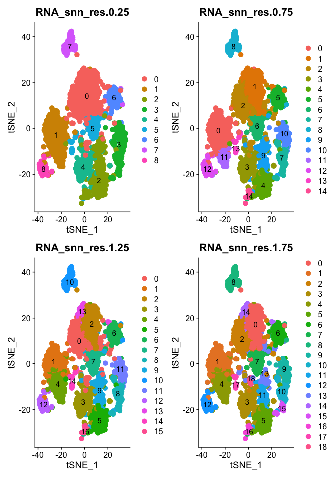
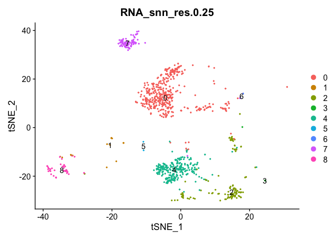
RNA_snn_res.0.25 RNA_snn_res.0.75 RNA_snn_res.1.25 RNA_snn_res.1.75 9 15 16 19 RNA_snn_res.2.25 RNA_snn_res.2.75 RNA_snn_res.3.25 RNA_snn_res.3.75 21 24 26 29

Plot TSNE coloring for each resolution

tSNE dimensionality reduction plots are then used to visualize clustering results. As input to the tSNE, you should use the same PCs as input to the clustering analysis.

experiment.aggregate <- RunTSNE(
  object = experiment.aggregate,
  reduction.use = "pca",
  dims = use.pcs,
  do.fast = TRUE)

DimPlot(object = experiment.aggregate, group.by=grep("res",colnames(experiment.aggregate@meta.data),value = TRUE)[1:4], ncol=2 , pt.size=3.0, reduction = "tsne", label = T)

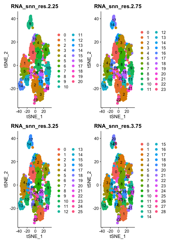
DimPlot(object = experiment.aggregate, group.by=grep("res",colnames(experiment.aggregate@meta.data),value = TRUE)[5:8], ncol=2 , pt.size=3.0, reduction = "tsne", label = T)

Try exploring different PCS, so first 5, 15, 25, we used 50, what about 100? How does the clustering change?

Once complete go back to 1:50

Choosing a resolution

Lets set the default identity to a resolution of 0.25 and produce a table of cluster to sample assignments.

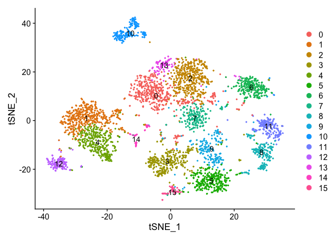
Idents(experiment.aggregate) <- "RNA_snn_res.1.25"
table(Idents(experiment.aggregate),experiment.aggregate$orig.ident)

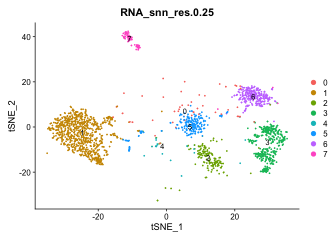
PBMC2 PBMC3 T021PBMC T022PBMC 0 19 19 341 90 1 43 403 3 7 2 9 0 15 431 3 7 15 284 49 4 15 315 10 5 5 7 2 76 219 6 247 13 2 0 7 203 2 0 6 8 12 179 2 13 9 150 6 30 18 10 73 10 92 29 11 171 12 1 0 12 0 0 37 99 13 6 0 87 5 14 33 24 2 3 15 5 0 18 26

Plot TSNE coloring by the slot ‘ident’ (default).

DimPlot(object = experiment.aggregate, pt.size=0.5, reduction = "tsne", label = T)

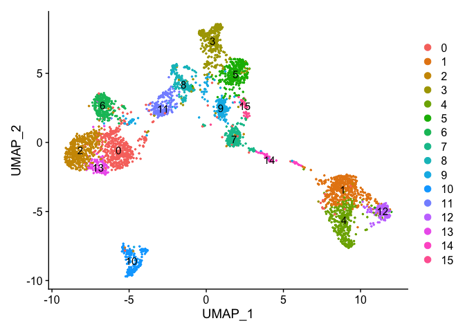
uMAP dimensionality reduction plot.

experiment.aggregate <- RunUMAP(
  object = experiment.aggregate,
  dims = use.pcs)

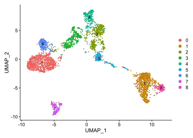
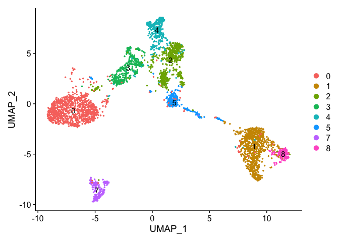
Plot uMap coloring by the slot ‘ident’ (default).

DimPlot(object = experiment.aggregate, pt.size=0.5, reduction = "umap", label = T)

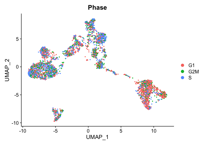
Catagorical data can be plotted using the DimPlot function.

TSNE plot by cell cycle

DimPlot(object = experiment.aggregate, pt.size=0.5, group.by = "Phase", reduction = "umap" )

Try creating a table, of cluster x cell cycle

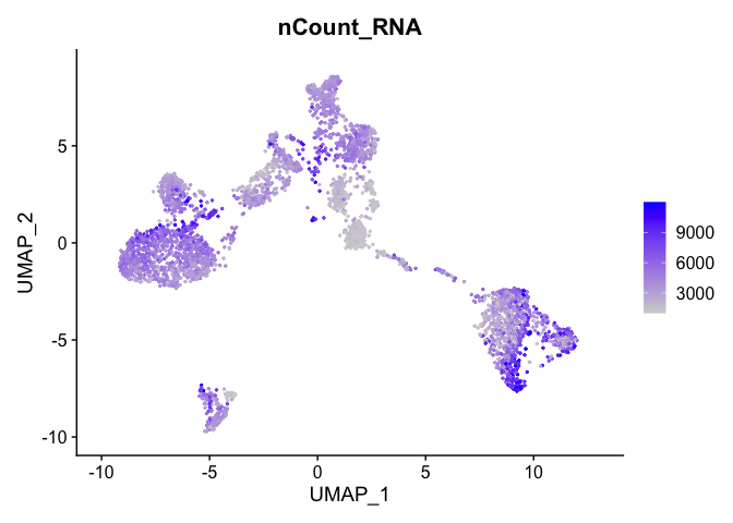
Can use feature plot to plot our read valued metadata, like nUMI, Feature count, and percent Mito

FeaturePlot can be used to color cells with a ‘feature’, non categorical data, like number of UMIs

FeaturePlot(experiment.aggregate, features = c('nCount_RNA'), pt.size=0.5)

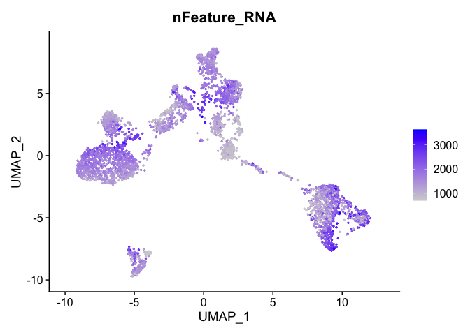
and number of genes present

FeaturePlot(experiment.aggregate, features = c('nFeature_RNA'), pt.size=0.5)

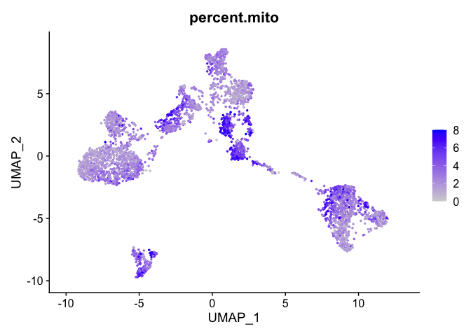
percent mitochondrial

FeaturePlot(experiment.aggregate, features = c('percent.mito'), pt.size=0.5)

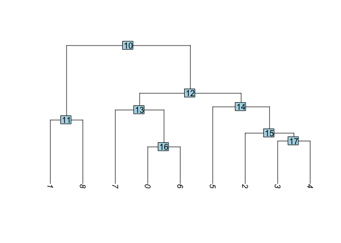
Building a phylogenetic tree relating the ‘average’ cell from each group in default ‘Ident’ (currently “RNA_snn_res.0.25”). Tree is estimated based on a distance matrix constructed in either gene expression space or PCA space.

Idents(experiment.aggregate) <- "RNA_snn_res.0.25"
experiment.aggregate <- BuildClusterTree(
  experiment.aggregate, dims = use.pcs)

PlotClusterTree(experiment.aggregate)

Create new trees of other data

Once complete go back to Res 0.25

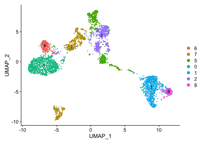
DimPlot(object = experiment.aggregate, pt.size=0.5, label = TRUE, reduction = "umap")

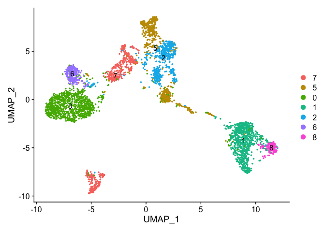
Merging clusters

Merge Clustering results, so lets say clusters 3 and 7 are actually the same cell type (overlaps in the tsne, not as apparent in the umap) and we don’t wish to separate them out as distinct clusters. Same with 4 and 5.

experiment.merged = experiment.aggregate
Idents(experiment.merged) <- "RNA_snn_res.0.25"

experiment.merged <- RenameIdents(
  object = experiment.merged,
  '3' = '7', '4' = '5'
)

table(Idents(experiment.merged))

7 5 0 1 2 6 8 595 627 1024 803 552 265 134

DimPlot(object = experiment.merged, pt.size=0.5, label = T, reduction = "umap")

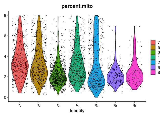
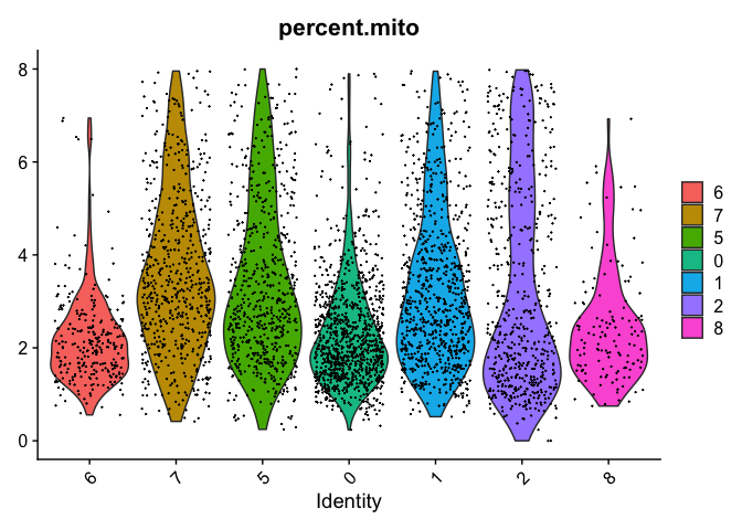
VlnPlot(object = experiment.merged, features = "percent.mito", pt.size = 0.05)

Reording the clusters

In order to reorder the clusters for plotting purposes take a look at the levels of the Ident, which indicates the ordering, then relevel as desired.

experiment.examples <- experiment.merged
levels(experiment.examples@active.ident)

[1] "7" "5" "0" "1" "2" "6" "8"

experiment.examples@active.ident <- relevel(experiment.examples@active.ident, "6")
levels(experiment.examples@active.ident)

[1] "6" "7" "5" "0" "1" "2" "8"

# now cluster 6 is the "first" factor

DimPlot(object = experiment.examples, pt.size=0.5, label = T, reduction = "umap")

VlnPlot(object = experiment.examples, features = "percent.mito", pt.size = 0.05)

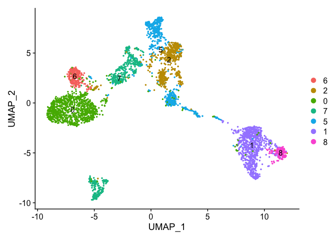
# relevel all the factors to the order I want
Idents(experiment.examples) <- factor(experiment.examples@active.ident, levels=c("6","2","0","7","5","9","1","8"))
levels(experiment.examples@active.ident)

[1] "6" "2" "0" "7" "5" "1" "8"

DimPlot(object = experiment.examples, pt.size=0.5, label = T, reduction = "umap")

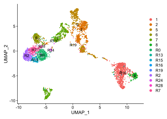
Re-assign clustering result (subclustering only cluster 0) to clustering for resolution 3.75 (@ reslution 0.25) [adding a R prefix]

newIdent = as.character(Idents(experiment.examples))
newIdent[newIdent == '0'] = paste0("R",as.character(experiment.examples$RNA_snn_res.3.75[newIdent == '0']))

Idents(experiment.examples) <- as.factor(newIdent)
table(Idents(experiment.examples))

1 2 5 6 7 8 R0 R13 R15 R16 R19 R2 R24 R28 R7 803 552 627 265 595 134 337 1 111 4 4 297 41 3 226

DimPlot(object = experiment.examples, pt.size=0.5, label = T, reduction = "umap")

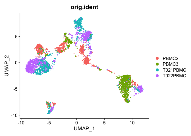
Plot UMAP coloring by the slot ‘orig.ident’ (sample names) with alpha colors turned on. A pretty picture

DimPlot(object = experiment.aggregate, group.by="orig.ident", pt.size=0.5, reduction = "umap" )

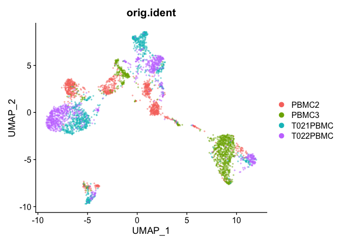
## Pretty umap using alpha
alpha.use <- 2/5
p <- DimPlot(object = experiment.aggregate, group.by="orig.ident", pt.size=0.5, reduction = "umap")
p$layers[[1]]$mapping$alpha <- alpha.use
p + scale_alpha_continuous(range = alpha.use, guide = F)

Removing cells assigned to clusters from a plot, So here plot all clusters but cluster 6 (contaminant?)

# create a new tmp object with those removed
experiment.aggregate.tmp <- experiment.aggregate[,-which(Idents(experiment.aggregate) %in% c("6"))]

dim(experiment.aggregate)

[1] 36601 4000

dim(experiment.aggregate.tmp)

[1] 36601 3735

DimPlot(object = experiment.aggregate.tmp, pt.size=0.5, reduction = "umap", label = T)

Identifying Marker Genes

Seurat can help you find markers that define clusters via differential expression.

FindMarkers identifies markers for a cluster relative to all other clusters.

FindAllMarkers does so for all clusters

FindAllMarkersNode defines all markers that split a Node from the cluster tree

?FindMarkers

markers = FindMarkers(experiment.aggregate, ident.1=c(3,7), ident.2 = c(4,5))

head(markers)

p_val avg_log2FC pct.1 pct.2 p_val_adj RPL13 6.509849e-128 1.266628 0.993 0.941 2.382670e-123 RPS5 5.564534e-107 1.375955 0.966 0.740 2.036675e-102 RPS19 8.747659e-104 1.214465 0.985 0.860 3.201731e-99 RPS8 5.925264e-102 1.128725 0.993 0.901 2.168706e-97 RPL29 3.151857e-93 1.075348 0.982 0.829 1.153611e-88 RPS18 3.693614e-93 1.170980 0.985 0.871 1.351900e-88

dim(markers)

[1] 1509 5

table(markers$avg_log2FC > 0)

FALSE TRUE 1002 507

table(markers$p_val_adj < 0.05 & markers$avg_log2FC > 0)

FALSE TRUE 1130 379

pct.1 and pct.2 are the proportion of cells with expression above 0 in ident.1 and ident.2 respectively. p_val is the raw p_value associated with the differntial expression test with adjusted value in p_val_adj. avg_logFC is the average log fold change difference between the two groups.

avg_diff (lines 130, 193 and) appears to be the difference in log(x = mean(x = exp(x = x) - 1) + 1) between groups. It doesn’t seem like this should work out to be the signed ratio of pct.1 to pct.2 so I must be missing something. It doesn’t seem to be related at all to how the p-values are calculated so maybe it doesn’t matter so much, and the sign is probably going to be pretty robust to how expression is measured.

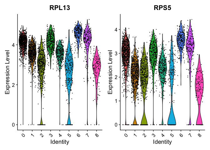
Can use a violin plot to visualize the expression pattern of some markers

VlnPlot(object = experiment.aggregate, features = rownames(markers)[1:2], pt.size = 0.05)

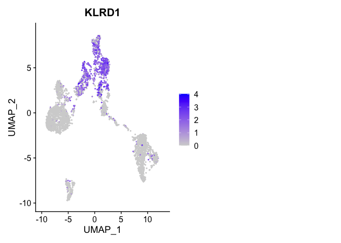
Or a feature plot

FeaturePlot(
    experiment.aggregate,
    "KLRD1",
    cols = c("lightgrey", "blue"),
    ncol = 2
)

FindAllMarkers can be used to automate the process across all genes.

markers_all <- FindAllMarkers(
    object = experiment.merged,
    only.pos = TRUE,
    min.pct = 0.25,
    thresh.use = 0.25
)
dim(markers_all)

[1] 4031 7

head(markers_all)

table(table(markers_all$gene))

1 2 3 4 1371 1049 178 7

markers_all_single <- markers_all[markers_all$gene %in% names(table(markers_all$gene))[table(markers_all$gene) == 1],]

dim(markers_all_single)

[1] 1371 7

table(table(markers_all_single$gene))

1 1371

table(markers_all_single$cluster)

7 5 0 1 2 6 8 45 24 151 325 520 70 236

head(markers_all_single)

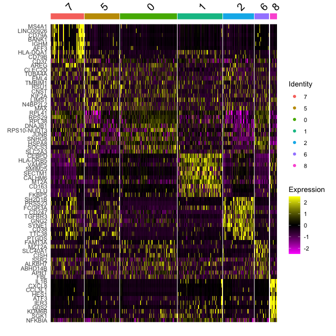
Plot a heatmap of genes by cluster for the top 10 marker genes per cluster

top10 <- markers_all_single %>% group_by(cluster) %>% top_n(10, avg_log2FC)
DoHeatmap(
    object = experiment.merged,
    features = top10$gene
)

# Get expression of genes for cells in and out of each cluster
getGeneClusterMeans <- function(gene, cluster){
  x <- GetAssayData(experiment.merged)[gene,]
  m <- tapply(x, ifelse(Idents(experiment.merged) == cluster, 1, 0), mean)
  mean.in.cluster <- m[2]
  mean.out.of.cluster <- m[1]
  return(list(mean.in.cluster = mean.in.cluster, mean.out.of.cluster = mean.out.of.cluster))
}

## for sake of time only using first six (head)
means <- mapply(getGeneClusterMeans, head(markers_all[,"gene"]), head(markers_all[,"cluster"]))
means <- matrix(unlist(means), ncol = 2, byrow = T)

colnames(means) <- c("mean.in.cluster", "mean.out.of.cluster")
rownames(means) <- head(markers_all[,"gene"])
markers_all2 <- cbind(head(markers_all), means)
head(markers_all2)

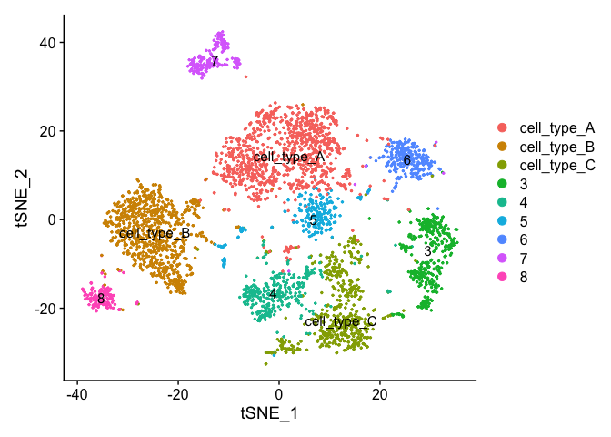
p_val avg_log2FC pct.1 pct.2 p_val_adj cluster gene MS4A1 7.868239e-202 2.460640 0.333 0.014 2.879854e-197 7 MS4A1 LINC00926 1.243988e-201 1.881382 0.292 0.005 4.553122e-197 7 LINC00926 CD79A 2.998365e-173 2.941748 0.336 0.024 1.097432e-168 7 CD79A BANK1 2.474993e-155 1.334570 0.255 0.009 9.058720e-151 7 BANK1 IGHM 1.796692e-143 1.835100 0.289 0.021 6.576072e-139 7 IGHM AFF3 6.026634e-129 1.291855 0.257 0.018 2.205808e-124 7 AFF3 mean.in.cluster mean.out.of.cluster MS4A1 0.8339190 0.020402330 LINC00926 0.6112367 0.008039788 CD79A 0.9998699 0.034222701 BANK1 0.4698104 0.012849977 IGHM 0.6230881 0.033921560 AFF3 0.4629120 0.023382292

Finishing up clusters.

At this point in time you should use the tree, markers, domain knowledge, and goals to finalize your clusters. This may mean adjusting PCA to use, mergers clusters together, choosing a new resolutions, etc. When finished you can further name it cluster by something more informative. Ex.

experiment.clusters <- experiment.aggregate
experiment.clusters <- RenameIdents(
  object = experiment.clusters,
  '0' = 'cell_type_A',
  '1' = 'cell_type_B',
  '2' = 'cell_type_C'
)
# and so on

DimPlot(object = experiment.clusters, pt.size=0.5, label = T, reduction = "tsne")

Right now our results ONLY exist in the Ident data object, lets save it to our metadata table so we don’t accidentally loose it.

experiment.merged$finalcluster <- Idents(experiment.merged)
head(experiment.merged[[]])

Subsetting samples and plotting

If you want to look at the representation of just one sample, or sets of samples

experiment.sample2 <- subset(experiment.merged, orig.ident == "T021PBMC")

DimPlot(object = experiment.sample2, group.by = "RNA_snn_res.0.25", pt.size=0.5, label = TRUE, reduction = "tsne")

experiment.batch1 <- subset(experiment.merged, batchid == "Batch1")

DimPlot(object = experiment.batch1, group.by = "RNA_snn_res.0.25", pt.size=0.5, label = TRUE, reduction = "tsne")

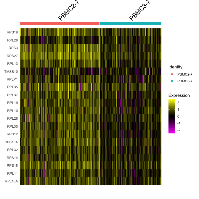
Adding in a new metadata column representing samples within clusters. So differential expression of PBMC2 vs PBMC3 within cluster 7

experiment.merged$samplecluster = paste(experiment.merged$orig.ident,experiment.merged$finalcluster,sep = '-')

# set the identity to the new variable
Idents(experiment.merged) <- "samplecluster"

markers.comp <- FindMarkers(experiment.merged, ident.1 = c("PBMC2-7","PBMC3-7"), ident.2= "PBMC2-5")

head(markers.comp)

p_val avg_log2FC pct.1 pct.2 p_val_adj RPS19 4.133527e-86 2.281703 0.983 0.725 1.512912e-81 RPL28 2.638843e-85 2.088881 0.987 0.749 9.658429e-81 RPS3 4.573010e-83 1.877041 0.993 0.814 1.673767e-78 RPS27 5.062436e-83 1.947372 0.991 0.870 1.852902e-78 RPL13 6.204595e-82 1.776009 0.991 0.931 2.270944e-77 TMSB10 2.145713e-80 1.909817 0.985 0.846 7.853524e-76

experiment.subset <- subset(experiment.merged, samplecluster %in%  c( "PBMC2-7", "PBMC3-7" ))
DoHeatmap(experiment.subset, features = head(rownames(markers.comp),20))

Idents(experiment.merged) <- "finalcluster"

And last lets save all the objects in our session.

save(list=ls(), file="clusters_seurat_object.RData")

Get the next Rmd file

download.file("https://raw.githubusercontent.com/ucdavis-bioinformatics-training/2021-March-Single-Cell-RNA-Seq-Analysis/master/data_analysis/scRNA_Workshop-PART6.Rmd", "scRNA_Workshop-PART6.Rmd")

Session Information

sessionInfo()

R version 4.0.3 (2020-10-10) Platform: x86_64-apple-darwin17.0 (64-bit) Running under: macOS Big Sur 10.16 Matrix products: default BLAS: /Library/Frameworks/R.framework/Versions/4.0/Resources/lib/libRblas.dylib LAPACK: /Library/Frameworks/R.framework/Versions/4.0/Resources/lib/libRlapack.dylib locale: [1] en_US.UTF-8/en_US.UTF-8/en_US.UTF-8/C/en_US.UTF-8/en_US.UTF-8 attached base packages: [1] stats graphics grDevices utils datasets methods base other attached packages: [1] dplyr_1.0.5 ggplot2_3.3.3 SeuratObject_4.0.0 Seurat_4.0.1 loaded via a namespace (and not attached): [1] Rtsne_0.15 colorspace_2.0-0 deldir_0.2-10 [4] ellipsis_0.3.1 ggridges_0.5.3 spatstat.data_2.1-0 [7] leiden_0.3.7 listenv_0.8.0 farver_2.1.0 [10] ggrepel_0.9.1 RSpectra_0.16-0 fansi_0.4.2 [13] codetools_0.2-18 splines_4.0.3 knitr_1.31 [16] polyclip_1.10-0 jsonlite_1.7.2 ica_1.0-2 [19] cluster_2.1.1 png_0.1-7 uwot_0.1.10 [22] shiny_1.6.0 sctransform_0.3.2 spatstat.sparse_2.0-0 [25] compiler_4.0.3 httr_1.4.2 assertthat_0.2.1 [28] Matrix_1.3-2 fastmap_1.1.0 lazyeval_0.2.2 [31] limma_3.44.3 later_1.1.0.1 htmltools_0.5.1.1 [34] tools_4.0.3 igraph_1.2.6 gtable_0.3.0 [37] glue_1.4.2 RANN_2.6.1 reshape2_1.4.4 [40] Rcpp_1.0.6 scattermore_0.7 jquerylib_0.1.3 [43] vctrs_0.3.6 ape_5.4-1 nlme_3.1-152 [46] lmtest_0.9-38 xfun_0.22 stringr_1.4.0 [49] globals_0.14.0 mime_0.10 miniUI_0.1.1.1 [52] lifecycle_1.0.0 irlba_2.3.3 goftest_1.2-2 [55] future_1.21.0 MASS_7.3-53.1 zoo_1.8-9 [58] scales_1.1.1 spatstat.core_2.0-0 promises_1.2.0.1 [61] spatstat.utils_2.1-0 parallel_4.0.3 RColorBrewer_1.1-2 [64] yaml_2.2.1 reticulate_1.18 pbapply_1.4-3 [67] gridExtra_2.3 sass_0.3.1 rpart_4.1-15 [70] stringi_1.5.3 highr_0.8 rlang_0.4.10 [73] pkgconfig_2.0.3 matrixStats_0.58.0 evaluate_0.14 [76] lattice_0.20-41 ROCR_1.0-11 purrr_0.3.4 [79] tensor_1.5 patchwork_1.1.1 htmlwidgets_1.5.3 [82] labeling_0.4.2 cowplot_1.1.1 tidyselect_1.1.0 [85] parallelly_1.24.0 RcppAnnoy_0.0.18 plyr_1.8.6 [88] magrittr_2.0.1 R6_2.5.0 generics_0.1.0 [91] DBI_1.1.1 pillar_1.5.1 withr_2.4.1 [94] mgcv_1.8-34 fitdistrplus_1.1-3 survival_3.2-10 [97] abind_1.4-5 tibble_3.1.0 future.apply_1.7.0 [100] crayon_1.4.1 KernSmooth_2.23-18 utf8_1.2.1 [103] spatstat.geom_2.0-1 plotly_4.9.3 rmarkdown_2.7 [106] grid_4.0.3 data.table_1.14.0 digest_0.6.27 [109] xtable_1.8-4 tidyr_1.1.3 httpuv_1.5.5 [112] munsell_0.5.0 viridisLite_0.3.0 bslib_0.2.4

☰ Menu

Single Cell RNA-Seq Analysis