☰ Menu

      RNA-Seq Analysis

Home
Introduction and Lectures
Intro to the Workshop and Core
Schedule
What is Bioinformatics/Genomics?
Experimental Design and Cost Estimation
RNA Sequencing Technologies - Dr. Lutz Froenicke
Support
Zoom
Slack
Cheat Sheets
Software and Links
Scripts
Prerequisites
CLI
R
Data Reduction
Files and Filetypes
Prepare dataset
Preprocessing raw data
Indexing a Genome
Alignment with Star
Generating counts tables
Alignment/Counts with Salmon (Extra)
3' TagSeq
Data analysis
Prepare R for data analysis
Annotation from BioMart
Differential Expression Analysis
Pathway Analysis
Comparison between STAR and Salmon
ETC
Closing thoughts
Workshop Photos
Github page
Report Errors
Biocore website

GO AND KEGG Enrichment Analysis

Load libraries

library(topGO)
Loading required package: BiocGenerics
Attaching package: 'BiocGenerics'
The following objects are masked from 'package:stats': IQR, mad, sd, var, xtabs
The following objects are masked from 'package:base': anyDuplicated, append, as.data.frame, basename, cbind, colnames, dirname, do.call, duplicated, eval, evalq, Filter, Find, get, grep, grepl, intersect, is.unsorted, lapply, Map, mapply, match, mget, order, paste, pmax, pmax.int, pmin, pmin.int, Position, rank, rbind, Reduce, rownames, sapply, setdiff, sort, table, tapply, union, unique, unsplit, which.max, which.min
Loading required package: graph
Loading required package: Biobase
Welcome to Bioconductor Vignettes contain introductory material; view with 'browseVignettes()'. To cite Bioconductor, see 'citation("Biobase")', and for packages 'citation("pkgname")'.
Loading required package: GO.db
Loading required package: AnnotationDbi
Loading required package: stats4
Loading required package: IRanges
Loading required package: S4Vectors
Attaching package: 'S4Vectors'
The following objects are masked from 'package:base': expand.grid, I, unname
Attaching package: 'IRanges'
The following object is masked from 'package:grDevices': windows
Loading required package: SparseM
Attaching package: 'SparseM'
The following object is masked from 'package:base': backsolve
groupGOTerms: GOBPTerm, GOMFTerm, GOCCTerm environments built.
Attaching package: 'topGO'
The following object is masked from 'package:IRanges': members
library(KEGGREST)
library(org.Mm.eg.db)
library(pathview)
Pathview is an open source software package distributed under GNU General Public License version 3 (GPLv3). Details of GPLv3 is available at http://www.gnu.org/licenses/gpl-3.0.html. Particullary, users are required to formally cite the original Pathview paper (not just mention it) in publications or products. For details, do citation("pathview") within R. The pathview downloads and uses KEGG data. Non-academic uses may require a KEGG license agreement (details at http://www.kegg.jp/kegg/legal.html).
library(ggplot2)

Files for examples were created in the DE analysis.

Gene Ontology (GO) Enrichment

Gene ontology provides a controlled vocabulary for describing biological processes (BP ontology), molecular functions (MF ontology) and cellular components (CC ontology)

The GO ontologies themselves are organism-independent; terms are associated with genes for a specific organism through direct experimentation or through sequence homology with another organism and its GO annotation.

Terms are related to other terms through parent-child relationships in a directed acylic graph.

Enrichment analysis provides one way of drawing conclusions about a set of differential expression results.

1. topGO Example Using Kolmogorov-Smirnov Testing Our first example uses Kolmogorov-Smirnov Testing for enrichment testing of our mouse DE results, with GO annotation obtained from the Bioconductor database org.Mm.eg.db.

The first step in each topGO analysis is to create a topGOdata object. This contains the genes, the score for each gene (here we use the p-value from the DE test), the GO terms associated with each gene, and the ontology to be used (here we use the biological process ontology)

infile <- "WT.C_v_WT.NC.txt"
tmp <- read.delim(infile)

geneList <- tmp$P.Value
xx <- as.list(org.Mm.egENSEMBL2EG)
names(geneList) <- xx[sapply(strsplit(tmp$Gene,split="\\."),"[[", 1L)]
head(geneList)
67241 68891 12772 70686 94212 219140 4.383027e-19 3.423886e-18 3.945562e-18 5.384455e-17 7.758438e-17 8.489480e-17
# Create topGOData object
GOdata <- new("topGOdata",
	ontology = "BP",
	allGenes = geneList,
	geneSelectionFun = function(x)x,
	annot = annFUN.org , mapping = "org.Mm.eg.db")
Building most specific GOs .....
( 10461 GO terms found. )
Build GO DAG topology ..........
( 14058 GO terms and 31916 relations. )
Annotating nodes ...............
( 10378 genes annotated to the GO terms. )

2. The topGOdata object is then used as input for enrichment testing:

# Kolmogorov-Smirnov testing
resultKS <- runTest(GOdata, algorithm = "weight01", statistic = "ks")
-- Weight01 Algorithm -- the algorithm is scoring 14058 nontrivial nodes parameters: test statistic: ks score order: increasing
Level 20: 1 nodes to be scored (0 eliminated genes)
Level 19: 8 nodes to be scored (0 eliminated genes)
Level 18: 17 nodes to be scored (1 eliminated genes)
Level 17: 38 nodes to be scored (29 eliminated genes)
Level 16: 82 nodes to be scored (64 eliminated genes)
Level 15: 178 nodes to be scored (135 eliminated genes)
Level 14: 350 nodes to be scored (333 eliminated genes)
Level 13: 622 nodes to be scored (747 eliminated genes)
Level 12: 1083 nodes to be scored (1633 eliminated genes)
Level 11: 1558 nodes to be scored (3210 eliminated genes)
Level 10: 1946 nodes to be scored (4707 eliminated genes)
Level 9: 2077 nodes to be scored (5893 eliminated genes)
Level 8: 1955 nodes to be scored (7085 eliminated genes)
Level 7: 1725 nodes to be scored (7939 eliminated genes)
Level 6: 1255 nodes to be scored (8647 eliminated genes)
Level 5: 690 nodes to be scored (9067 eliminated genes)
Level 4: 324 nodes to be scored (9314 eliminated genes)
Level 3: 126 nodes to be scored (9428 eliminated genes)
Level 2: 22 nodes to be scored (9477 eliminated genes)
Level 1: 1 nodes to be scored (9506 eliminated genes)
tab <- GenTable(GOdata, raw.p.value = resultKS, topNodes = length(resultKS@score), numChar = 120)

topGO by default preferentially tests more specific terms, utilizing the topology of the GO graph. The algorithms used are described in detail here.

head(tab, 15)
GO.ID Term 1 GO:0045087 innate immune response 2 GO:0045944 positive regulation of transcription by RNA polymerase II 3 GO:0045766 positive regulation of angiogenesis 4 GO:0045071 negative regulation of viral genome replication 5 GO:0032731 positive regulation of interleukin-1 beta production 6 GO:0051897 positive regulation of protein kinase B signaling 7 GO:0031623 receptor internalization 8 GO:0008360 regulation of cell shape 9 GO:0032760 positive regulation of tumor necrosis factor production 10 GO:0051607 defense response to virus 11 GO:0008150 biological_process 12 GO:0006002 fructose 6-phosphate metabolic process 13 GO:0007229 integrin-mediated signaling pathway 14 GO:0070374 positive regulation of ERK1 and ERK2 cascade 15 GO:0001525 angiogenesis Annotated Significant Expected raw.p.value 1 530 530 530 4.0e-10 2 768 768 768 3.7e-08 3 97 97 97 2.8e-07 4 49 49 49 4.8e-07 5 51 51 51 1.2e-06 6 61 61 61 1.3e-06 7 79 79 79 1.6e-06 8 105 105 105 1.6e-06 9 85 85 85 1.9e-06 10 228 228 228 2.0e-06 11 10378 10378 10378 2.6e-06 12 10 10 10 3.2e-06 13 63 63 63 6.4e-06 14 108 108 108 6.6e-06 15 300 300 300 7.3e-06

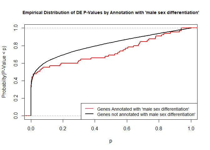
The Kolmogorov-Smirnov test directly compares two probability distributions based on their maximum distance.

To illustrate the KS test, we plot probability distributions of p-values that are and that are not annotated with the term GO:0046661 “male sex differentiation” (66 genes) p-value 0.8721. (This won’t exactly match what topGO does due to their elimination algorithm):

rna.pp.terms <- genesInTerm(GOdata)[["GO:0046661"]] # get genes associated with term
p.values.in <- geneList[names(geneList) %in% rna.pp.terms]
p.values.out <- geneList[!(names(geneList) %in% rna.pp.terms)]
plot.ecdf(p.values.in, verticals = T, do.points = F, col = "red", lwd = 2, xlim = c(0,1),
          main = "Empirical Distribution of DE P-Values by Annotation with 'male sex differentiation'",
          cex.main = 0.9, xlab = "p", ylab = "Probabilty(P-Value < p)")
ecdf.out <- ecdf(p.values.out)
xx <- unique(sort(c(seq(0, 1, length = 201), knots(ecdf.out))))
lines(xx, ecdf.out(xx), col = "black", lwd = 2)
legend("bottomright", legend = c("Genes Annotated with 'male sex differentiation'", "Genes not annotated with male sex differentiation'"), lwd = 2, col = 2:1, cex = 0.9)

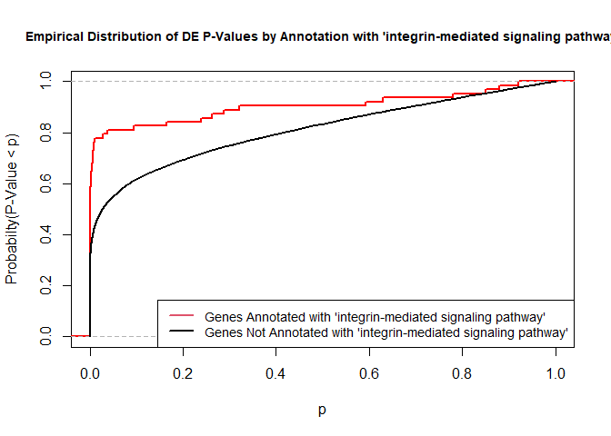
versus the probability distributions of p-values that are and that are not annotated with the term GO:0007229 “integrin-mediated signaling pathway” (66 genes) p-value 9.8x10⁻⁵.

rna.pp.terms <- genesInTerm(GOdata)[["GO:0007229"]] # get genes associated with term
p.values.in <- geneList[names(geneList) %in% rna.pp.terms]
p.values.out <- geneList[!(names(geneList) %in% rna.pp.terms)]
plot.ecdf(p.values.in, verticals = T, do.points = F, col = "red", lwd = 2, xlim = c(0,1),
          main = "Empirical Distribution of DE P-Values by Annotation with 'integrin-mediated signaling pathway'",
          cex.main = 0.9, xlab = "p", ylab = "Probabilty(P-Value < p)")
ecdf.out <- ecdf(p.values.out)
xx <- unique(sort(c(seq(0, 1, length = 201), knots(ecdf.out))))
lines(xx, ecdf.out(xx), col = "black", lwd = 2)
legend("bottomright", legend = c("Genes Annotated with 'integrin-mediated signaling pathway'", "Genes Not Annotated with 'integrin-mediated signaling pathway'"), lwd = 2, col = 2:1, cex = 0.9)

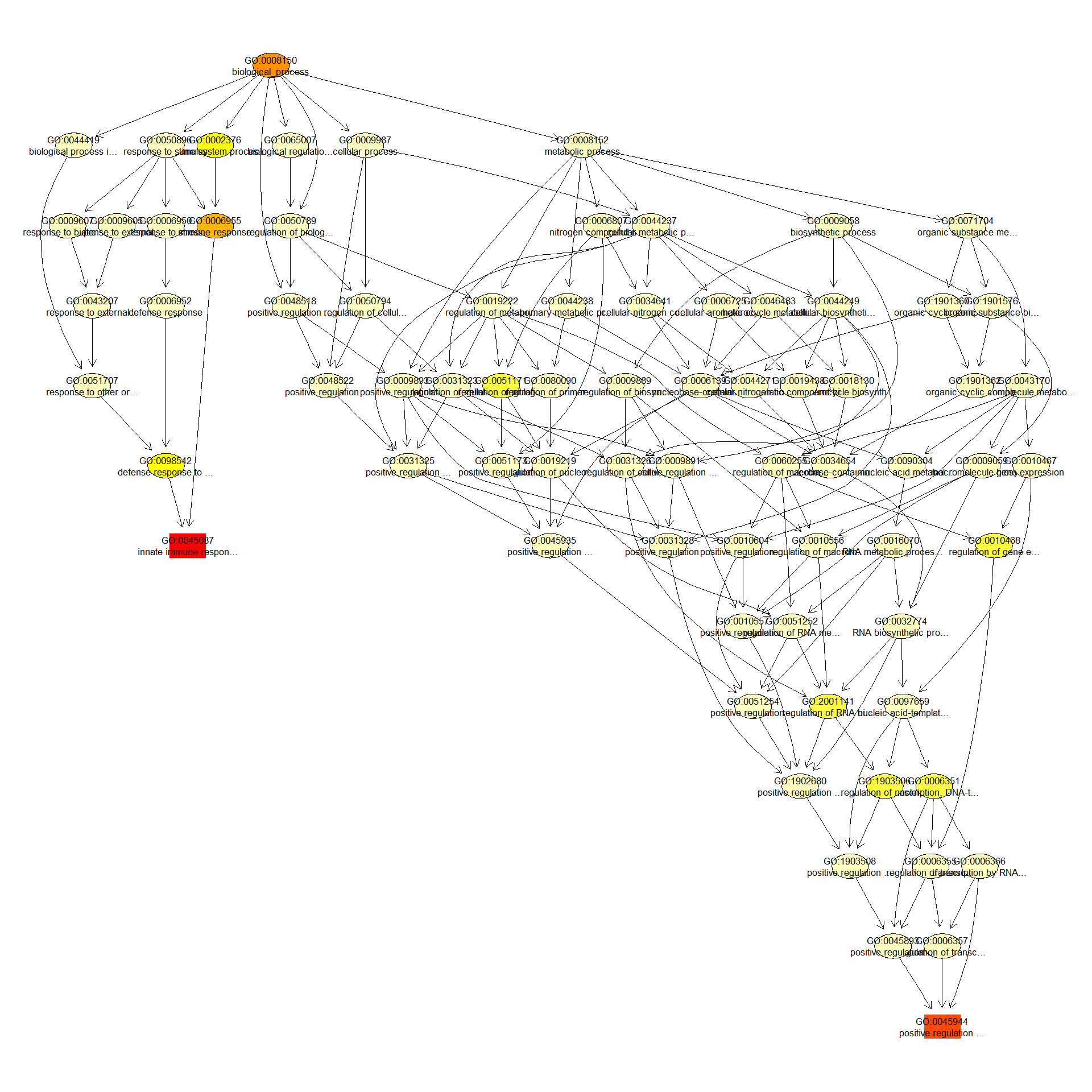
We can use the function showSigOfNodes to plot the GO graph for the 3 most significant terms and their parents, color coded by enrichment p-value (red is most significant):

par(cex = 0.3)
showSigOfNodes(GOdata, score(resultKS), firstSigNodes = 2, useInfo = "def")
Loading required package: Rgraphviz
Loading required package: grid
Attaching package: 'grid'
The following object is masked from 'package:topGO': depth
Attaching package: 'Rgraphviz'
The following objects are masked from 'package:IRanges': from, to
The following objects are masked from 'package:S4Vectors': from, to

$dag A graphNEL graph with directed edges Number of Nodes = 74 Number of Edges = 161 $complete.dag [1] "A graph with 74 nodes."
par(cex = 1)

3. topGO Example Using Fisher’s Exact Test

Next, we use Fisher’s exact test to test for GO enrichment among significantly DE genes.

Create topGOdata object:

# Create topGOData object
GOdata <- new("topGOdata",
	ontology = "BP",
	allGenes = geneList,
	geneSelectionFun = function(x) (x < 0.05),
	annot = annFUN.org , mapping = "org.Mm.eg.db")
Building most specific GOs .....
( 10461 GO terms found. )
Build GO DAG topology ..........
( 14058 GO terms and 31916 relations. )
Annotating nodes ...............
( 10378 genes annotated to the GO terms. )

Run Fisher’s Exact Test:

resultFisher <- runTest(GOdata, algorithm = "elim", statistic = "fisher")
-- Elim Algorithm -- the algorithm is scoring 12736 nontrivial nodes parameters: test statistic: fisher cutOff: 0.01
Level 20: 1 nodes to be scored (0 eliminated genes)
Level 19: 8 nodes to be scored (0 eliminated genes)
Level 18: 17 nodes to be scored (0 eliminated genes)
Level 17: 35 nodes to be scored (0 eliminated genes)
Level 16: 73 nodes to be scored (19 eliminated genes)
Level 15: 158 nodes to be scored (94 eliminated genes)
Level 14: 304 nodes to be scored (94 eliminated genes)
Level 13: 521 nodes to be scored (304 eliminated genes)
Level 12: 935 nodes to be scored (1549 eliminated genes)
Level 11: 1378 nodes to be scored (1842 eliminated genes)
Level 10: 1761 nodes to be scored (2046 eliminated genes)
Level 9: 1901 nodes to be scored (2563 eliminated genes)
Level 8: 1790 nodes to be scored (3184 eliminated genes)
Level 7: 1586 nodes to be scored (3935 eliminated genes)
Level 6: 1159 nodes to be scored (4759 eliminated genes)
Level 5: 657 nodes to be scored (5360 eliminated genes)
Level 4: 308 nodes to be scored (5995 eliminated genes)
Level 3: 121 nodes to be scored (6573 eliminated genes)
Level 2: 22 nodes to be scored (6729 eliminated genes)
Level 1: 1 nodes to be scored (6729 eliminated genes)
tab <- GenTable(GOdata, raw.p.value = resultFisher, topNodes = length(resultFisher@score),
				numChar = 120)
head(tab)
GO.ID Term 1 GO:0045087 innate immune response 2 GO:0042742 defense response to bacterium 3 GO:0045944 positive regulation of transcription by RNA polymerase II 4 GO:0001525 angiogenesis 5 GO:0032760 positive regulation of tumor necrosis factor production 6 GO:0032731 positive regulation of interleukin-1 beta production Annotated Significant Expected raw.p.value 1 530 364 298.90 2.0e-08 2 165 126 93.05 5.8e-08 3 768 497 433.13 6.5e-07 4 300 223 169.19 6.9e-06 5 85 67 47.94 1.2e-05 6 51 43 28.76 2.1e-05

Fisher’s Exact Test is applied to the table:

Significance/Annotation Annotated With GO Term Not Annotated With GO Term
Significantly DE n1 n3
Not Significantly DE n2 n4

and compares the probability of the observed table, conditional on the row and column sums, to what would be expected under random chance.

Advantages over KS (or Wilcoxon) Tests:

Disadvantages:

Quiz 1

KEGG Pathway Enrichment Testing With KEGGREST

KEGG, the Kyoto Encyclopedia of Genes and Genomes (https://www.genome.jp/kegg/), provides assignment of genes for many organisms into pathways.

We will access KEGG pathway assignments for mouse through the KEGGREST Bioconductor package, and then use some homebrew code for enrichment testing.

1. Get all mouse pathways and their genes:

# Pull all pathways for mmu
pathways.list <- keggList("pathway", "mmu")
head(pathways.list)
path:mmu00010 "Glycolysis / Gluconeogenesis - Mus musculus (house mouse)" path:mmu00020 "Citrate cycle (TCA cycle) - Mus musculus (house mouse)" path:mmu00030 "Pentose phosphate pathway - Mus musculus (house mouse)" path:mmu00040 "Pentose and glucuronate interconversions - Mus musculus (house mouse)" path:mmu00051 "Fructose and mannose metabolism - Mus musculus (house mouse)" path:mmu00052 "Galactose metabolism - Mus musculus (house mouse)"
# Pull all genes for each pathway
pathway.codes <- sub("path:", "", names(pathways.list))
genes.by.pathway <- sapply(pathway.codes,
	function(pwid){
		pw <- keggGet(pwid)
		if (is.null(pw[[1]]$GENE)) return(NA)
		pw2 <- pw[[1]]$GENE[c(TRUE,FALSE)] # may need to modify this to c(FALSE, TRUE) for other organisms
		pw2 <- unlist(lapply(strsplit(pw2, split = ";", fixed = T), function(x)x[1]))
		return(pw2)
	}
)
head(genes.by.pathway)
$mmu00010 [1] "15277" "212032" "15275" "216019" "103988" "14751" [7] "18641" "18642" "56421" "14121" "14120" "11674" [13] "230163" "11676" "353204" "79459" "21991" "14433" [19] "115487111" "14447" "18655" "18663" "18648" "56012" [25] "13806" "13807" "13808" "433182" "226265" "18746" [31] "18770" "18597" "18598" "68263" "235339" "13382" [37] "16828" "16832" "16833" "106557" "11522" "11529" [43] "26876" "11532" "58810" "11669" "11671" "72535" [49] "110695" "56752" "11670" "67689" "621603" "73458" [55] "68738" "60525" "319625" "72157" "66681" "14377" [61] "14378" "68401" "72141" "12183" "17330" "18534" [67] "74551" $mmu00020 [1] "12974" "71832" "104112" "11429" "11428" "15926" "269951" "15929" [9] "67834" "170718" "243996" "18293" "239017" "78920" "13382" "56451" [17] "20917" "20916" "66945" "67680" "66052" "66925" "14194" "17449" [25] "17448" "18563" "18534" "74551" "18597" "18598" "68263" "235339" $mmu00030 [1] "14751" "14380" "14381" "66171" "100198" "110208" "66646" "21881" [9] "83553" "74419" "21351" "19895" "232449" "71336" "72157" "66681" [17] "19139" "110639" "328099" "75456" "19733" "75731" "235582" "11674" [25] "230163" "11676" "353204" "79459" "14121" "14120" "18641" "18642" [33] "56421" $mmu00040 [1] "110006" "16591" "22238" "22236" "94284" "94215" "394434" "394430" [9] "394432" "394433" "72094" "552899" "71773" "394435" "394436" "100727" [17] "231396" "100559" "112417" "243085" "613123" "22235" "216558" "58810" [25] "68631" "66646" "102448" "11997" "14187" "11677" "67861" "67880" [33] "20322" "71755" "75578" "75847" $mmu00051 [1] "110119" "54128" "29858" "331026" "69080" "218138" "22122" "75540" [9] "234730" "15277" "212032" "15275" "216019" "18641" "18642" "56421" [17] "14121" "14120" "18639" "18640" "170768" "270198" "319801" "16548" [25] "20322" "11997" "14187" "11677" "67861" "11674" "230163" "11676" [33] "353204" "79459" "21991" "225913" $mmu00052 [1] "319625" "14635" "14430" "74246" "216558" "72157" "66681" "15277" [9] "212032" "15275" "216019" "103988" "14377" "14378" "68401" "12091" [17] "226413" "16770" "14595" "53418" "11605" "11997" "14187" "11677" [25] "67861" "18641" "18642" "56421" "232714" "14387" "76051" "69983"

Read in DE file to be used in enrichment testing:

head(geneList)
67241 68891 12772 70686 94212 219140 4.383027e-19 3.423886e-18 3.945562e-18 5.384455e-17 7.758438e-17 8.489480e-17

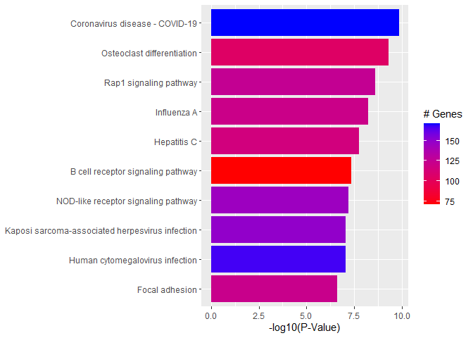
2. Apply Wilcoxon rank-sum test to each pathway, testing if “in” p-values are smaller than “out” p-values:

# Wilcoxon test for each pathway
pVals.by.pathway <- t(sapply(names(genes.by.pathway),
	function(pathway) {
		pathway.genes <- genes.by.pathway[[pathway]]
		list.genes.in.pathway <- intersect(names(geneList), pathway.genes)
		list.genes.not.in.pathway <- setdiff(names(geneList), list.genes.in.pathway)
		scores.in.pathway <- geneList[list.genes.in.pathway]
		scores.not.in.pathway <- geneList[list.genes.not.in.pathway]
		if (length(scores.in.pathway) > 0){
			p.value <- wilcox.test(scores.in.pathway, scores.not.in.pathway, alternative = "less")$p.value
		} else{
			p.value <- NA
		}
		return(c(p.value = p.value, Annotated = length(list.genes.in.pathway)))
	}
))

# Assemble output table
outdat <- data.frame(pathway.code = rownames(pVals.by.pathway))
outdat$pathway.name <- pathways.list[paste0("path:",outdat$pathway.code)]
outdat$p.value <- pVals.by.pathway[,"p.value"]
outdat$Annotated <- pVals.by.pathway[,"Annotated"]
outdat <- outdat[order(outdat$p.value),]
head(outdat)
pathway.code pathway.name 300 mmu05171 Coronavirus disease - COVID-19 - Mus musculus (house mouse) 169 mmu04380 Osteoclast differentiation - Mus musculus (house mouse) 121 mmu04015 Rap1 signaling pathway - Mus musculus (house mouse) 293 mmu05164 Influenza A - Mus musculus (house mouse) 289 mmu05160 Hepatitis C - Mus musculus (house mouse) 196 mmu04662 B cell receptor signaling pathway - Mus musculus (house mouse) p.value Annotated 300 1.464505e-10 171 169 5.084974e-10 105 121 2.585792e-09 125 293 6.055844e-09 121 289 1.844962e-08 116 196 4.710489e-08 71

The Wilcoxon rank-sum test is the nonparametric analogue of the two-sample t-test. It compares the ranks of observations in two groups. It is more powerful than the Kolmogorov-Smirnov test.

3. Plotting Pathways

foldChangeList <- tmp$logFC
xx <- as.list(org.Mm.egENSEMBL2EG)
names(foldChangeList) <- xx[sapply(strsplit(tmp$Gene,split="\\."),"[[", 1L)]
head(foldChangeList)
67241 68891 12772 70686 94212 219140 -2.487719 4.552564 2.164336 -4.121437 -1.899178 -2.676304
mmu04380 <- pathview(gene.data  = foldChangeList,
                     pathway.id = "mmu04380",
                     species    = "mmu",
                     limit      = list(gene=max(abs(foldChangeList)), cpd=1))
'select()' returned 1:1 mapping between keys and columns
Info: Working in directory C:/Users/bpdurbin/Desktop/2022-June-RNA-Seq-Analysis/data_analysis
Info: Writing image file mmu04380.pathview.png

Barplot of p-values for top pathways

A barplot of -log10(p-value) for the top pathways can be used for any type of enrichment analysis.

plotdat <- outdat[1:10,]
plotdat$nice.name <- gsub(" - Mus musculus (house mouse)", "", plotdat$pathway.name, fixed = TRUE)

ggplot(plotdat, aes(x = -log10(p.value), y = reorder(nice.name, -log10(p.value)), fill = Annotated)) + geom_bar(stat = "identity") + labs(x = "-log10(P-Value)", y = NULL, fill = "# Genes") + scale_fill_gradient(low = "red", high = "blue")

Quiz 2

sessionInfo()
R version 4.2.0 (2022-04-22 ucrt) Platform: x86_64-w64-mingw32/x64 (64-bit) Running under: Windows 10 x64 (build 19044) Matrix products: default locale: [1] LC_COLLATE=English_United States.utf8 [2] LC_CTYPE=English_United States.utf8 [3] LC_MONETARY=English_United States.utf8 [4] LC_NUMERIC=C [5] LC_TIME=English_United States.utf8 attached base packages: [1] grid stats4 stats graphics grDevices utils datasets [8] methods base other attached packages: [1] Rgraphviz_2.40.0 ggplot2_3.3.6 pathview_1.36.0 [4] org.Mm.eg.db_3.15.0 KEGGREST_1.36.2 topGO_2.48.0 [7] SparseM_1.81 GO.db_3.15.0 AnnotationDbi_1.58.0 [10] IRanges_2.30.0 S4Vectors_0.34.0 Biobase_2.56.0 [13] graph_1.74.0 BiocGenerics_0.42.0 loaded via a namespace (and not attached): [1] KEGGgraph_1.56.0 Rcpp_1.0.8.3 lattice_0.20-45 [4] png_0.1-7 Biostrings_2.64.0 utf8_1.2.2 [7] digest_0.6.29 R6_2.5.1 GenomeInfoDb_1.32.2 [10] RSQLite_2.2.14 evaluate_0.15 highr_0.9 [13] httr_1.4.3 pillar_1.7.0 zlibbioc_1.42.0 [16] rlang_1.0.2 curl_4.3.2 jquerylib_0.1.4 [19] blob_1.2.3 rmarkdown_2.14 labeling_0.4.2 [22] stringr_1.4.0 RCurl_1.98-1.7 bit_4.0.4 [25] munsell_0.5.0 compiler_4.2.0 xfun_0.31 [28] pkgconfig_2.0.3 htmltools_0.5.2 tidyselect_1.1.2 [31] tibble_3.1.7 GenomeInfoDbData_1.2.8 matrixStats_0.62.0 [34] XML_3.99-0.10 fansi_1.0.3 withr_2.5.0 [37] dplyr_1.0.9 crayon_1.5.1 bitops_1.0-7 [40] jsonlite_1.8.0 gtable_0.3.0 lifecycle_1.0.1 [43] DBI_1.1.2 magrittr_2.0.3 scales_1.2.0 [46] cli_3.3.0 stringi_1.7.6 cachem_1.0.6 [49] farver_2.1.0 XVector_0.36.0 bslib_0.3.1 [52] generics_0.1.2 ellipsis_0.3.2 vctrs_0.4.1 [55] org.Hs.eg.db_3.15.0 tools_4.2.0 bit64_4.0.5 [58] glue_1.6.2 purrr_0.3.4 fastmap_1.1.0 [61] yaml_2.3.5 colorspace_2.0-3 memoise_2.0.1 [64] knitr_1.39 sass_0.4.1