
Quality checks in our data
Load our libraries
# Set up global options for nice reports and keeping figures:
knitr::opts_chunk$set(fig.width=14, fig.height=8, fig.align="center",
                      warning=FALSE, message=FALSE)
Lets start by loading libraries
library(phyloseq)
library(vegan)
library(ggplot2)
library(kableExtra)
library(tidyr)

nice_colors = c("#999999", "#E69F00", "#56B4E9","#e98756","#c08160","#5800e6", "#CDDC49", "#C475D3",
                "#E94B30", "#233F57", "#FEE659", "#A1CFDD", "#F4755E", "#D6F6F7","#EB6D58", "#6898BF")
Load prior results
load(file=file.path("rdata_objects", "initial_rooted.Rdata"))
Exploring reads, ASVs per sample
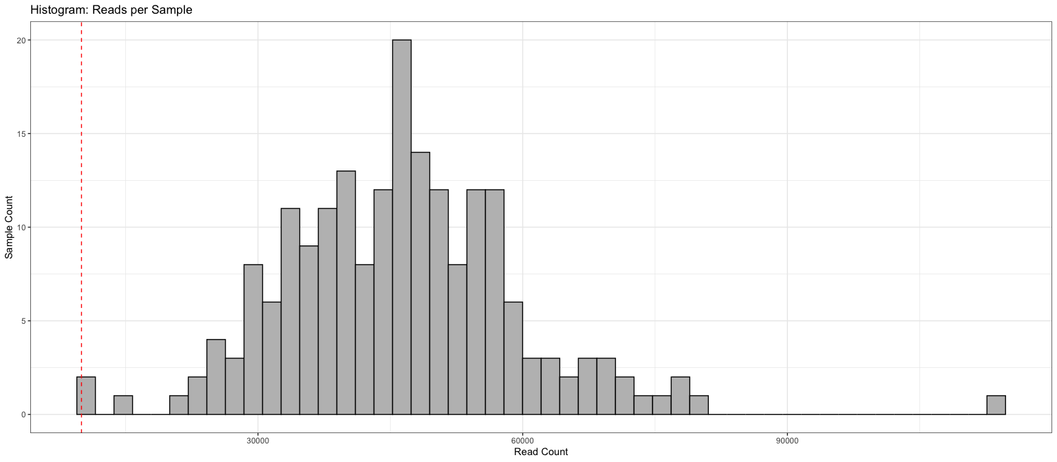
Reads per sample, all samples
df = data.frame(ASVs=rowSums(otu_table(ps)>0), reads=sample_sums(ps), sample_data(ps))

ggplot(df, aes(x=reads)) + geom_histogram(bins=50, color='black', fill='grey') +
  theme_bw() +  geom_vline(xintercept=10000, color= "red", linetype='dashed') +
  labs(title="Histogram: Reads per Sample") + xlab("Read Count") + ylab("Sample Count")
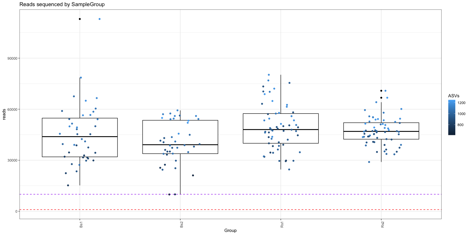
Scatter Plot, ASVs vs reads
ggplot(df, aes(x = Group, y = reads, color = ASVs)) +
  geom_boxplot(color="black") + theme_bw() +
  geom_jitter(width=.2, height=0)  +
  theme(axis.text.x = element_text(angle = 90)) +
  geom_hline(yintercept=10000, color= "purple", linetype='dashed') +
  geom_hline(yintercept=1000, color= "red", linetype='dashed') +
  ggtitle("Reads sequenced by SampleGroup")
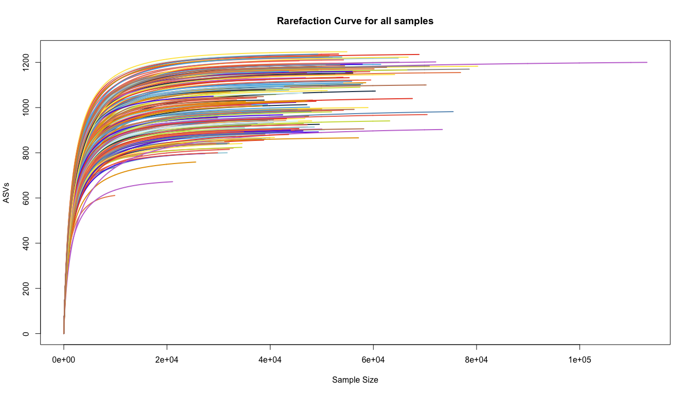
Rarefaction curve plots
Rarefaction curves show the number of Amplicon Sequence Variants detected as a function of sequencing depth. Optimally the curve will flatten out, indicating that most of the diversity in the population has been sampled. Depending on the type of experiment, it may not be necessary to fully sample the community in order to obtain useful information about the major changes or trends, especially for common community members.
out = rarecurve(otu_table(ps), col=nice_colors, step=100 , lwd=2, ylab="ASVs", label=F,
              main="Rarefaction Curve for all samples")
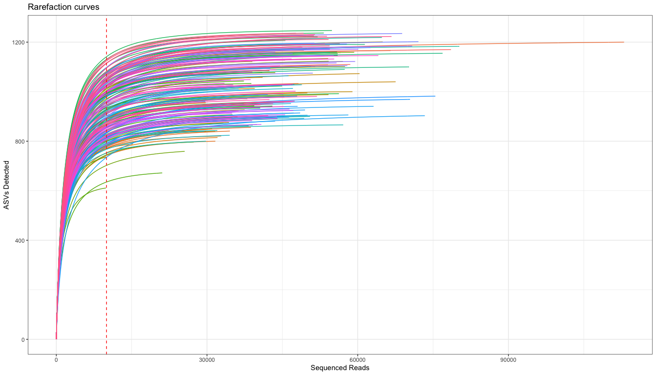
A ggplot rarefacion curve, borrowed form here
# We use the rarefaction curve data produce by vegan above
names(out) = rownames(otu_table(ps))

# Coerce data into "long" form.
protox <- mapply(FUN = function(x, y) {
  mydf <- as.data.frame(x)
  colnames(mydf) <- "value"
  mydf$SampleID <- y
  mydf$subsample <- attr(x, "Subsample")
  mydf
}, x = out, y = as.list(names(out)), SIMPLIFY = FALSE)

xy <- do.call(rbind, protox)
rownames(xy) <- NULL  # pretty
xy = data.frame(xy,
  sample_data(ps)[match(xy$SampleID, rownames(sample_data(ps))), ])
# Plot Rarefaction curve
ggplot(xy, aes(x = subsample, y = value, color = SampleID)) +
  theme_bw() +
  scale_color_discrete(guide = FALSE) +  # turn legend on or off
  geom_line() +
  geom_vline(xintercept=10000, color= "red", linetype='dashed') +
  labs(title="Rarefaction curves") + xlab("Sequenced Reads") + ylab('ASVs Detected')
# Plot Rarefaction curve
ggplot(xy, aes(x = subsample, y = value, color = SampleID)) +
  theme_bw() +
  scale_color_discrete(guide = FALSE) +  # turn legend on or off
  geom_line() +
  facet_wrap(~Group) +
  geom_vline(xintercept=10000, color= "red", linetype='dashed') +
  labs(title="Rarefaction curves by Group") + xlab("Sequenced Reads") + ylab('ASVs Detected')
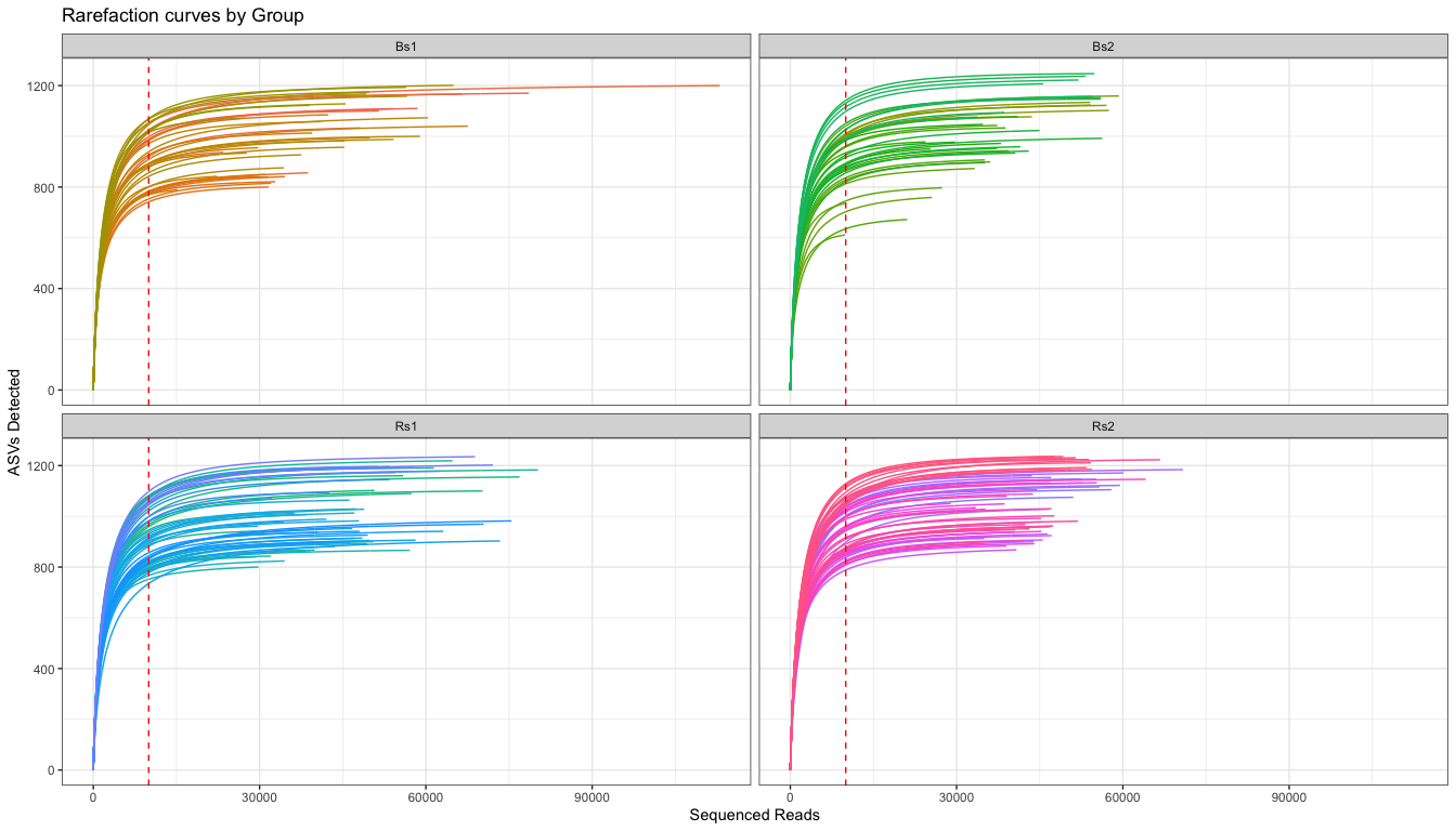
# Plot Rarefaction curve, faceting by group
ggplot(xy, aes(x = subsample, y = value, color = SampleID)) +
  theme_bw() +
  scale_color_discrete(guide = FALSE) +  # turn legend on or off
  geom_line() +
  facet_wrap(~Group) +
  geom_vline(xintercept=10000, color= "red", linetype='dashed') +
  labs(title="Rarefaction curves by Group") + xlab("Sequenced Reads") + ylab('ASVs Detected')

The rarefaction curves suggest that there is a range of ~800-1200 ASV per sample in the study. Each group is also pretty similar
- Try faceting by the Temperature, do you see a different trend?
Exploring the relationship between ASV and read count.
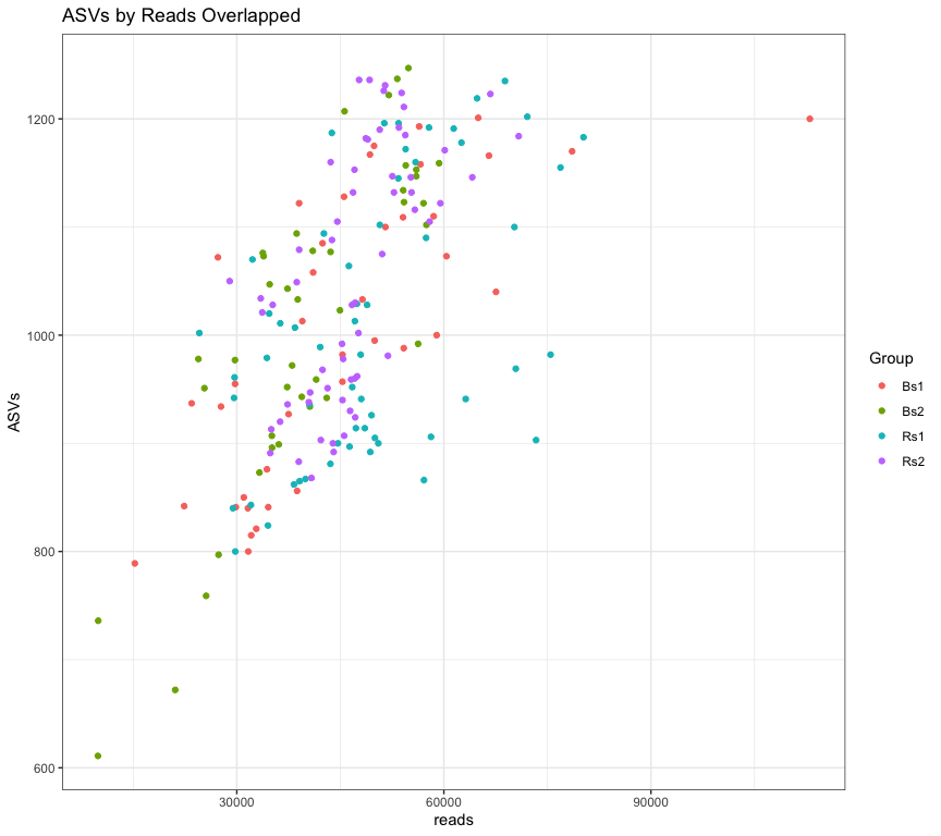 Scatter plot of ASVs by Reads colored by Group indicates that all samples mix well and are fairly well sampled.
- What about coloring by the other factors, Temp and Replicate? Do any new patterns emerge?
Taxonomic Assignment QA/QC
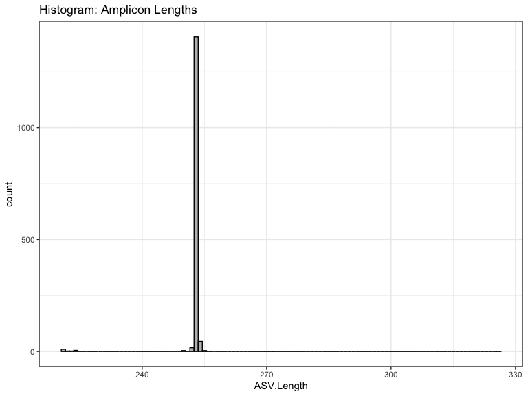
Plotting the amplicon length distribution
df = data.frame(names=names(refseq(ps)), ASV.Length = Biostrings::width(refseq(ps)))
ggplot(df, aes(x=ASV.Length)) + geom_histogram(binwidth=1, color='black', fill='grey') +
  theme_bw() + labs(title="Histogram: Amplicon Lengths")
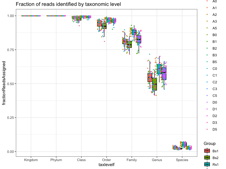
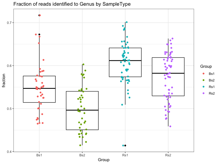
Are there trends in the fraction of reads that can be assigned to taxonomic level by experimental variables?
readsPerSample = rowSums(otu_table(ps))
fractionReadsAssigned = sapply(colnames(tax_table(ps)), function(x){
  rowSums(otu_table(ps)[, !is.na(tax_table(ps))[,x]]) / readsPerSample
})

fractionReadsAssigned = data.frame(SampleID = rownames(fractionReadsAssigned), fractionReadsAssigned)
fractionReadsAssigned.L = pivot_longer(fractionReadsAssigned,
    cols=colnames(tax_table(ps)), names_to="taxlevel", values_to="fractionReadsAssigned")
fractionReadsAssigned.L = data.frame(fractionReadsAssigned.L, sample_data(ps)[fractionReadsAssigned.L$SampleID,])

fractionReadsAssigned.L$taxlevelf = factor(fractionReadsAssigned.L$taxlevel, levels=c("Kingdom","Phylum","Class","Order","Family","Genus","Species"))

# Boxplot, fraction assigned by SampleType
ggplot(fractionReadsAssigned.L, aes(y = fractionReadsAssigned, x = taxlevelf, fill=Group, color=Replicate)) +
  theme_bw() +
  geom_boxplot(color='black', outlier.shape=NA) +
  ggtitle("Fraction of reads identified by taxonomic level") +
  geom_point(position=position_jitterdodge(jitter.width=0, jitter.height=0), size=.5)
Are there trends in the fraction of ASVs that can be assigned to taxonomic level by experimental variables?
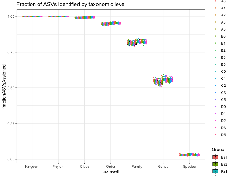
Genus level:
The statistics in this plot are calculated by merging taxa at the “Genus” rank with the tax_glom() function. This strategy works by summing reads from all ASVs with the same assignment at the specified taxonomic level. The ASV with the highest read count is selected as the representative for the agglomerated set. ASV with NA are removed.
Top 20 most abundant ASVs and their taxonomic assignment:
| Prevalence | TotalAbundance | Kingdom | Phylum | Class | Order | Family | Genus | Species | |
|---|---|---|---|---|---|---|---|---|---|
| ASV1 | 197 | 170379 | Bacteria | Desulfobacterota | Syntrophobacteria | Syntrophobacterales | Syntrophobacteraceae | Syntrophobacter | NA |
| ASV2 | 185 | 88391 | Bacteria | Cyanobacteria | Cyanobacteriia | Chloroplast | NA | NA | NA |
| ASV3 | 197 | 88231 | Bacteria | Firmicutes | Bacilli | Bacillales | Planococcaceae | Paenisporosarcina | NA |
| ASV4 | 197 | 51311 | Bacteria | Myxococcota | bacteriap25 | NA | NA | NA | NA |
| ASV5 | 195 | 47771 | Bacteria | Firmicutes | Bacilli | Bacillales | Planococcaceae | Paenisporosarcina | NA |
| ASV6 | 197 | 46828 | Bacteria | Firmicutes | Clostridia | Clostridiales | Clostridiaceae | Clostridium sensu stricto 1 | NA |
| ASV7 | 179 | 44661 | Bacteria | Bacteroidota | Bacteroidia | Chitinophagales | Chitinophagaceae | Flavisolibacter | NA |
| ASV8 | 148 | 43180 | Bacteria | Proteobacteria | Alphaproteobacteria | Rickettsiales | Mitochondria | NA | NA |
| ASV9 | 196 | 42622 | Bacteria | Firmicutes | Bacilli | Bacillales | Bacillaceae | Bacillus | NA |
| ASV10 | 196 | 41505 | Bacteria | Bacteroidota | Ignavibacteria | Ignavibacteriales | Ignavibacteriaceae | Ignavibacterium | NA |
| ASV11 | 166 | 38181 | Bacteria | Proteobacteria | Alphaproteobacteria | Rickettsiales | Mitochondria | NA | NA |
| ASV12 | 106 | 38181 | Bacteria | Proteobacteria | Alphaproteobacteria | Rickettsiales | Mitochondria | NA | NA |
| ASV13 | 166 | 37665 | Bacteria | Bacteroidota | Bacteroidia | Chitinophagales | Chitinophagaceae | NA | NA |
| ASV14 | 197 | 37063 | Bacteria | Desulfobacterota | Desulfuromonadia | Geobacterales | Geobacteraceae | Citrifermentans | NA |
| ASV15 | 187 | 35443 | Bacteria | Bacteroidota | Bacteroidia | Chitinophagales | Chitinophagaceae | NA | NA |
| ASV16 | 195 | 34794 | Bacteria | Actinobacteriota | Actinobacteria | Streptomycetales | Streptomycetaceae | Streptomyces | NA |
| ASV17 | 197 | 33384 | Bacteria | Bacteroidota | Bacteroidia | Chitinophagales | Chitinophagaceae | Flavisolibacter | NA |
| ASV18 | 197 | 33231 | Bacteria | Desulfobacterota | Desulfuromonadia | Geobacterales | Geobacteraceae | Geobacter | NA |
| ASV19 | 196 | 32304 | Bacteria | Firmicutes | Clostridia | Clostridiales | Clostridiaceae | Clostridium sensu stricto 1 | NA |
| ASV20 | 196 | 28475 | Bacteria | Actinobacteriota | Actinobacteria | Micrococcales | Micrococcaceae | Pseudarthrobacter | NA |
Top 20 most prevalent ASVs and their taxonomic assignment:
| Prevalence | TotalAbundance | Kingdom | Phylum | Class | Order | Family | Genus | Species | |
|---|---|---|---|---|---|---|---|---|---|
| ASV1 | 197 | 170379 | Bacteria | Desulfobacterota | Syntrophobacteria | Syntrophobacterales | Syntrophobacteraceae | Syntrophobacter | NA |
| ASV3 | 197 | 88231 | Bacteria | Firmicutes | Bacilli | Bacillales | Planococcaceae | Paenisporosarcina | NA |
| ASV4 | 197 | 51311 | Bacteria | Myxococcota | bacteriap25 | NA | NA | NA | NA |
| ASV6 | 197 | 46828 | Bacteria | Firmicutes | Clostridia | Clostridiales | Clostridiaceae | Clostridium sensu stricto 1 | NA |
| ASV14 | 197 | 37063 | Bacteria | Desulfobacterota | Desulfuromonadia | Geobacterales | Geobacteraceae | Citrifermentans | NA |
| ASV17 | 197 | 33384 | Bacteria | Bacteroidota | Bacteroidia | Chitinophagales | Chitinophagaceae | Flavisolibacter | NA |
| ASV18 | 197 | 33231 | Bacteria | Desulfobacterota | Desulfuromonadia | Geobacterales | Geobacteraceae | Geobacter | NA |
| ASV22 | 197 | 28145 | Bacteria | Cyanobacteria | Cyanobacteriia | Chloroplast | NA | NA | NA |
| ASV43 | 197 | 21056 | Bacteria | Nitrospirota | Thermodesulfovibrionia | NA | NA | NA | NA |
| ASV49 | 197 | 20157 | Bacteria | Desulfobacterota | Desulfobacteria | Desulfobacterales | Desulfosarcinaceae | Desulfatirhabdium | NA |
| ASV50 | 197 | 20143 | Bacteria | Proteobacteria | Alphaproteobacteria | Rickettsiales | Mitochondria | NA | NA |
| ASV52 | 197 | 19850 | Bacteria | Bacteroidota | Ignavibacteria | Ignavibacteriales | Ignavibacteriaceae | Ignavibacterium | NA |
| ASV53 | 197 | 19751 | Bacteria | Firmicutes | Clostridia | Clostridiales | Clostridiaceae | Clostridium sensu stricto 13 | NA |
| ASV59 | 197 | 19032 | Bacteria | Proteobacteria | Gammaproteobacteria | Burkholderiales | Comamonadaceae | Ramlibacter | NA |
| ASV61 | 197 | 18837 | Bacteria | Firmicutes | Bacilli | Bacillales | Planococcaceae | Planococcus | NA |
| ASV63 | 197 | 18705 | Bacteria | Desulfobacterota | Desulfuromonadia | Geobacterales | Geobacteraceae | NA | NA |
| ASV67 | 197 | 18273 | Bacteria | Desulfobacterota | Desulfuromonadia | Geobacterales | Geobacteraceae | NA | NA |
| ASV70 | 197 | 17907 | Bacteria | RCP2-54 | NA | NA | NA | NA | NA |
| ASV83 | 197 | 16694 | Bacteria | Desulfobacterota | Desulfuromonadia | Geobacterales | Geobacteraceae | Citrifermentans | NA |
| ASV92 | 197 | 15733 | Bacteria | Desulfobacterota | Syntrophobacteria | Syntrophobacterales | Syntrophobacteraceae | Desulfovirga | NA |
Cleanup
We haven’t edited our object yet, so no need to save it.
Get next Rmd
download.file("https://raw.githubusercontent.com/ucdavis-bioinformatics-training/2021-May-Microbial-Community-Analysis/master/data_analysis/mca_part3.Rmd", "mca_part3.Rmd")
Record session information
sessionInfo()
## R version 4.0.3 (2020-10-10)
## Platform: x86_64-apple-darwin17.0 (64-bit)
## Running under: macOS Big Sur 10.16
##
## Matrix products: default
## BLAS:   /Library/Frameworks/R.framework/Versions/4.0/Resources/lib/libRblas.dylib
## LAPACK: /Library/Frameworks/R.framework/Versions/4.0/Resources/lib/libRlapack.dylib
##
## locale:
## [1] en_US.UTF-8/en_US.UTF-8/en_US.UTF-8/C/en_US.UTF-8/en_US.UTF-8
##
## attached base packages:
## [1] stats     graphics  grDevices utils     datasets  methods   base
##
## other attached packages:
## [1] tidyr_1.1.3      kableExtra_1.3.4 ggplot2_3.3.3    vegan_2.5-7
## [5] lattice_0.20-44  permute_0.9-5    phyloseq_1.34.0
##
## loaded via a namespace (and not attached):
##  [1] Biobase_2.50.0      httr_1.4.2          sass_0.4.0
##  [4] viridisLite_0.4.0   jsonlite_1.7.2      splines_4.0.3
##  [7] foreach_1.5.1       bslib_0.2.5.1       assertthat_0.2.1
## [10] highr_0.9           stats4_4.0.3        yaml_2.2.1
## [13] progress_1.2.2      pillar_1.6.1        glue_1.4.2
## [16] digest_0.6.27       XVector_0.30.0      rvest_1.0.0
## [19] colorspace_2.0-1    htmltools_0.5.1.1   Matrix_1.3-3
## [22] plyr_1.8.6          pkgconfig_2.0.3     zlibbioc_1.36.0
## [25] purrr_0.3.4         webshot_0.5.2       scales_1.1.1
## [28] svglite_2.0.0       tibble_3.1.2        mgcv_1.8-35
## [31] farver_2.1.0        generics_0.1.0      IRanges_2.24.1
## [34] ellipsis_0.3.2      withr_2.4.2         BiocGenerics_0.36.1
## [37] survival_3.2-11     magrittr_2.0.1      crayon_1.4.1
## [40] evaluate_0.14       fansi_0.4.2         nlme_3.1-152
## [43] MASS_7.3-54         xml2_1.3.2          tools_4.0.3
## [46] data.table_1.14.0   prettyunits_1.1.1   hms_1.1.0
## [49] lifecycle_1.0.0     stringr_1.4.0       Rhdf5lib_1.12.1
## [52] S4Vectors_0.28.1    munsell_0.5.0       cluster_2.1.2
## [55] Biostrings_2.58.0   ade4_1.7-16         compiler_4.0.3
## [58] jquerylib_0.1.4     systemfonts_1.0.2   rlang_0.4.11
## [61] rhdf5_2.34.0        grid_4.0.3          iterators_1.0.13
## [64] rhdf5filters_1.2.1  biomformat_1.18.0   rstudioapi_0.13
## [67] igraph_1.2.6        labeling_0.4.2      rmarkdown_2.8
## [70] gtable_0.3.0        codetools_0.2-18    multtest_2.46.0
## [73] DBI_1.1.1           reshape2_1.4.4      R6_2.5.0
## [76] knitr_1.33          dplyr_1.0.6         utf8_1.2.1
## [79] ape_5.5             stringi_1.6.2       parallel_4.0.3
## [82] Rcpp_1.0.6          vctrs_0.3.8         tidyselect_1.1.1
## [85] xfun_0.23