
R and RStudio
What is R?
R is a language and environment for statistical computing and graphics developed in 1993. It provides a wide variety of statistical and graphical techniques (linear and nonlinear modeling, statistical tests, time series analysis, classification, clustering, …), and is highly extensible, meaning that the user community can write new R tools. It is a GNU project (Free and Open Source).
The R language has its roots in the S language and environment which was developed at Bell Laboratories (formerly AT&T, now Lucent Technologies) by John Chambers and colleagues. R was created by Ross Ihaka and Robert Gentleman at the University of Auckland, New Zealand, and now, R is developed by the R Development Core Team, of which Chambers is a member. R is named partly after the first names of the first two R authors (Robert Gentleman and Ross Ihaka), and partly as a play on the name of S. R can be considered as a different implementation of S. There are some important differences, but much code written for S runs unaltered under R.
Some of R’s strengths:
- The ease with which well-designed publication-quality plots can be produced, including mathematical symbols and formulae where needed. Great care has been taken over the defaults for the minor design choices in graphics, but the user retains full control.
- It compiles and runs on a wide variety of UNIX platforms and similar systems (including FreeBSD and Linux), Windows and MacOS.
- R can be extended (easily) via packages.
- R has its own LaTeX-like documentation format, which is used to supply comprehensive documentation, both on-line in a number of formats and in hardcopy.
- It has a vast community both in academia and in business.
- It’s FREE!
The R environment
R is an integrated suite of software facilities for data manipulation, calculation and graphical display. It includes
- an effective data handling and storage facility,
- a suite of operators for calculations on arrays, in particular matrices,
- a large, coherent, integrated collection of intermediate tools for data analysis,
- graphical facilities for data analysis and display either on-screen or on hardcopy, and
- a well-developed, and effective programming language which includes conditionals, loops, user-defined recursive functions and input and output facilities.
The term “environment” is intended to characterize it as a fully planned and coherent system, rather than an incremental accretion of very specific and inflexible tools, as is frequently the case with other data analysis software.
R, like S, is designed around a true computer language, and it allows users to add additional functionality by defining new functions. Much of the system is itself written in the R dialect of S, which makes it easy for users to follow the algorithmic choices made. For computationally-intensive tasks, C, C++ and Fortran code can be linked and called at run time. Advanced users can write C code to manipulate R objects directly.
Many users think of R as a statistics system. The R group prefers to think of it of an environment within which statistical techniques are implemented.
The R Homepage
The R homepage has a wealth of information on it,
On the homepage you can:
- Learn more about R
- Download R
- Get Documentation (official and user supplied)
- Get access to CRAN ‘Comprehensive R archival network’
Interface for R
There are many ways one can interface with R language. Here are a few popular ones:
RStudio
RStudio started in 2010, to offer R a more full featured integrated development environment (IDE) and modeled after matlab’s IDE.
RStudio has many features:
- syntax highlighting
- code completion
- smart indentation
- “Projects”
- workspace browser and data viewer
- embedded plots
- Markdown notebooks, Sweave authoring and knitr with one click pdf or html
- runs on all platforms and over the web
- etc. etc. etc.
RStudio and its team have contributed to many R packages.[13] These include:
- Tidyverse – R packages for data science, including ggplot2, dplyr, tidyr, and purrr
- Shiny – An interactive web technology
- RMarkdown – Insert R code into markdown documents
- knitr – Dynamic reports combining R, TeX, Markdown & HTML
- packrat – Package dependency tool
- devtools – Package development tool
RStudio Cheat Sheets: rstudio-ide.pdf
Topics covered in this introduction to R
- Basic concepts
- Basic data types in R
- Import and export data in R
- Functions in R
- Basic statistics in R
- Simple data visulization in R
- Install packages in R
- Save data in R session
Topic 1. Basic concepts
There are three concepts that we should be familiar with before working in R:
- Operators
| Operator | Description |
|---|---|
| <-, = | Assignment |
| Operator | Description |
|---|---|
| \+ | Addition |
| \- | Subtraction |
| \* | Multiplication |
| / | Division |
| ^ | Exponent |
| %% | Modulus |
| %/% | Integer Division |
| Operator | Description |
|---|---|
| < | Less than |
| > | Greater than |
| <= | Less than or equal to |
| >= | Greater than or equal to |
| == | Equal to |
| != | Not equal to |
| Operator | Description |
|---|---|
| ! | Logical NOT |
| & | Element-wise logical AND |
| && | Logical AND |
| | | Element-wise logical OR |
| || | Logical OR |
- Functions
Functions are essential in all programming languages. A function takes zero or more parameters and return a result. The way to use a function in R is:
function.name(parameter1=value1, …)
- Variables
A variable is a named storage. The name of a variable can have letters, numbers, dot and underscore. However, a valid variable name cannot start with a underscore or a number, or start with a dot that is followed by a number.
Topic 2. Basic data types in R
Simple variables: variables that have a numeric value, a character value (such as a string), or a logical value (True or False)
Examples of numeric values.
# assign number 150 to variable a.
a <- 150
a
# assign a number in scientific format to variable b.
b <- 3e-2
b
Examples of character values.
# assign a string "Professor" to variable title
title <- "Professor"
title
# assign a string "Hello World" to variable hello
hello <- "Hello World"
hello
Examples of logical values.
# assign logical value "TRUE" to variable is_female
is_female <- TRUE
is_female
# assign logical value "FALSE" to variable is_male
is_male <- FALSE
is_male
# assign logical value to a variable by logical operation
age <- 20
is_adult <- age > 18
is_adult
To find out the type of variable.
class(is_female)
# To check whether the variable is a specific type
is.numeric(hello)
is.numeric(a)
is.character(hello)
The rule to convert a logical variable to numeric: TRUE > 1, FALSE > 0
as.numeric(is_female)
as.numeric(is_male)
R does not know how to convert a numeric variable to a character variable.
b
as.character(b)
Vectors: a vector is a combination of multiple values(numeric, character or logical) in the same object. A vector is created using the function c() (for concatenate).
friend_ages <- c(21, 27, 26, 32)
friend_ages
friend_names <- c("Mina", "Ella", "Anna", "Cora")
friend_names
One can give names to the elements of a vector.
# assign names to a vector by specifying them
names(friend_ages) <- c("Mina", "Ella", "Anna", "Carla")
friend_ages
# assign names to a vector using another vector
names(friend_ages) <- friend_names
friend_ages
Or One may create a vector with named elements from scratch.
friend_ages <- c(Mina=21, Ella=27, Anna=26, Cora=32)
friend_ages
To find out the length of a vector:
length(friend_ages)
To access elements of a vector: by index, or by name if it is a named vector.
friend_ages[2]
friend_ages["Ella"]
friend_ages[c(1,3)]
friend_ages[c("Mina", "Anna")]
# selecting elements of a vector by excluding some of them.
friend_ages[-3]
To select a subset of a vector can be done by logical vector.
my_friends <- c("Mina", "Ella", "Anna", "Cora")
my_friends
has_child <- c("TRUE", "TRUE", "FALSE", "TRUE")
has_child
my_friends[has_child == "TRUE"]
NOTE: a vector can only hold elements of the same type.
Matrices: A matrix is like an Excel sheet containing multiple rows and columns. It is used to combine vectors of the same type.
col1 <- c(1,3,8,9)
col2 <- c(2,18,27,10)
col3 <- c(8,37,267,19)

my_matrix <- cbind(col1, col2, col3)
my_matrix
rownames(my_matrix) <- c("row1", "row2", "row3", "row4")
my_matrix
t(my_matrix)
To find out the dimension of a matrix:
ncol(my_matrix)
nrow(my_matrix)
dim(my_matrix)
Accessing elements of a matrix is done in similar ways to accessing elements of a vector.
my_matrix[1,3]
my_matrix["row1", "col3"]
my_matrix[1,]
my_matrix[,3]
my_matrix[col3 > 20,]
Calculations with matrices.
my_matrix * 3
log10(my_matrix)
Total of each row.
rowSums(my_matrix)
Total of each column.
colSums(my_matrix)
It is also possible to use the function apply() to apply any statistical functions to rows/columns of matrices. The advantage of using apply() is that it can take a function created by user.
The simplified format of apply() is as following:
apply(X, MARGIN, FUN)
X: data matrix MARGIN: possible values are 1 (for rows) and 2 (for columns) FUN: the function to apply on rows/columns
To calculate the mean of each row.
apply(my_matrix, 1, mean)
To calculate the median of each row
apply(my_matrix, 1, median)
Factors: a factor represents categorical or groups in data. The function factor() can be used to create a factor variable.
friend_groups <- factor(c(1,2,1,2))
friend_groups
In R, categories are called factor levels. The function levels() can be used to access the factor levels.
levels(friend_groups)
Change the factor levels.
levels(friend_groups) <- c("best_friend", "not_best_friend")
friend_groups
Change the order of levels.
levels(friend_groups) <- c("not_best_friend", "best_friend")
friend_groups
By default, the order of factor levels is taken in the order of numeric or alphabetic.
friend_groups <- factor(c("not_best_friend", "best_friend", "not_best_friend", "best_friend"))
friend_groups
The factor levels can be specified when creating the factor, if the order does not follow the default rule.
friend_groups <- factor(c("not_best_friend", "best_friend", "not_best_friend", "best_friend"), levels=c("not_best_friend", "best_friend"))
friend_groups
If you want to know the number of individuals at each levels, there are two functions.
summary(friend_groups)
table(friend_groups)
Data frames: a data frame is like a matrix but can have columns with different types (numeric, character, logical).
A data frame can be created using the function data.frame().
# creating a data frame using previously defined vectors
friends <- data.frame(name=friend_names, age=friend_ages, child=has_child)
friends
To check whether a data is a data frame, use the function is.data.frame().
is.data.frame(friends)
is.data.frame(my_matrix)
One can convert a object to a data frame using the function as.data.frame().
class(my_matrix)
my_data <- as.data.frame(my_matrix)
class(my_data)
A data frame can be transposed in the similar way as a matrix.
my_data
t(my_data)
To obtain a subset of a data frame can be done in similar ways as we have discussed: by index, by row/column names, or by logical values.
friends["Mina",]
# The columns of a data frame can be referred to by the names of the columns
friends
friends$age
friends[friends$age > 26,]
friends[friends$child == "TRUE",]
Function subset() can also be used to get a subset of a data frame.
# select friends that are older than 26
subset(friends, age > 26)
# select the information of the ages of friends
subset(friends, select=age)
A data frame can be extended.
# add a column that has the information on the marrital status of friends
friends$married <- c("YES", "YES", "NO", "YES")
friends
A data frame can also be extended using the functions cbind() and rbind().
# add a column that has the information on the salaries of friends
cbind(friends, salary=c(4000, 8000, 2000, 6000))
Lists: a list is an ordered collection of objects, which can be any type of R objects (vectors, matrices, data frames).
A list can be created using the function list().
my_list <- list(mother="Sophia", father="John", sisters=c("Anna", "Emma"), sister_age=c(5, 10))
my_list
# names of elements in the list
names(my_list)
# number of elements in the list
length(my_list)
To access elements of a list can be done using its name or index.
my_list$mother
my_list[["mother"]]
my_list[[1]]
my_list[[3]]
my_list[[3]][2]
Topic 3. Import and export data in R
R base function read.table() is a general funciton that can be used to read a file in table format. The data will be imported as a data frame.
# To read a local file. If you have downloaded the raw_counts.txt file to your local machine, you may use the following command to read it in, by providing the full path for the file location. The way to specify the full path is the same as taught in the command line session. Here we assume raw_counts.txt is in our current working directory
data <- read.table(file="./Intro2R_files/raw_counts.txt", sep="\t", header=T, stringsAsFactors=F)

# There is a very convenient way to read files from the internet.
data <- read.table(file="https://raw.githubusercontent.com/ucdavis-bioinformatics-training/2019_August_UCD_mRNAseq_Workshop/master/intro2R/Intro2R_files/raw_counts.txt", sep="\t", header=T, stringsAsFactors=F)
Take a look at the beginning part of the data frame.
head(data)
Depending on the format of the file, several variants of read.table() are available to make reading a file easier.
read.csv(): for reading “comma separated value” files (.csv).
read.csv2(): variant used in countries that use a comma “,” as decimal point and a semicolon “;” as field separators.
read.delim(): for reading “tab separated value” files (“.txt”). By default, point(“.”) is used as decimal point.
read.delim2(): for reading “tab separated value” files (“.txt”). By default, comma (“,”) is used as decimal point.
# We are going to read a file over the internet by providing the url of the file.
data2 <- read.csv(file="https://raw.githubusercontent.com/ucdavis-bioinformatics-training/2019_August_UCD_mRNAseq_Workshop/master/intro2R/Intro2R_files/raw_counts.txt", stringsAsFactors=F)

# To look at the file:
head(data2)
R base function write.table() can be used to export data to a file.
# To write to a file called "output.txt" in your current working directory.
write.table(data2[1:20,], file="output.txt", sep="\t", quote=F, row.names=T, col.names=T)
It is also possible to export data to a csv file.
write.csv()
write.csv2()
\newpage
Topic 4. Functions in R
Invoking a function by its name, followed by the parenthesis and zero or more arguments.
# to find out the current working directory
getwd()
# to set a different working directory, use setwd
#setwd("/Users/jli/Desktop")

# to list all variables in the environment
ls()
# to create a vector from 2 to 3, using increment of 0.1
seq(2, 3, by=0.1)
# to create a vector with repeated elements
rep(1:3, times=3)
rep(1:3, each=3)
# to get help information on a function in R: ?function.name
?seq
?sort
?rep
str(data2)
Two special functions: lapply() and sapply()
lapply() is to apply a given function to every element of a vector and obtain a list as results. The difference between lapply() and apply() is that lapply() can be applied on objects like dataframes, lists or vectors. Function apply() only works on an array of dimension 2 or a matrix.
To check the syntax of using lapply():
#?lapply()

data <- as.data.frame(matrix(rnorm(49), ncol=7), stringsAsFactors=F)
dim(data)
lapply(1:dim(data)[1], function(x){sum(data[x,])})
apply(data, MARGIN=1, sum)
lapply(1:dim(data)[1], function(x){log10(sum(data[x,]))})
The function sapply() works like function lapply(), but tries to simplify the output to the most elementary data structure that is possible. As a matter of fact, sapply() is a “wrapper” function for lapply(). By default, it returns a vector.
# To check the syntax of using sapply():
#?sapply()

sapply(1:dim(data)[1], function(x){log10(sum(data[x,]))})
If the “simplify” parameter is turned off, sapply() will produced exactly the same results as lapply(), in the form of a list. By default, “simplify” is turned on.
sapply(1:dim(data)[1], function(x){log10(sum(data[x,]))}, simplify=FALSE)
Topic 5. Basic statistics in R
| Description | R_function |
|---|---|
| Mean | mean() |
| Standard deviation | sd() |
| Variance | var() |
| Minimum | min() |
| Maximum | max() |
| Median | median() |
| Range of values: minimum and maximum | range() |
| Sample quantiles | quantile() |
| Generic function | summary() |
| Interquartile range | IQR() |
Calculate the mean expression for each sample.
apply(data, 2, mean)
Calculate the range of expression for each sample.
apply(data, 2, range)
Calculate the quantiles of each samples.
apply(data, 2, quantile)
Topic 6. Simple data visulization in R
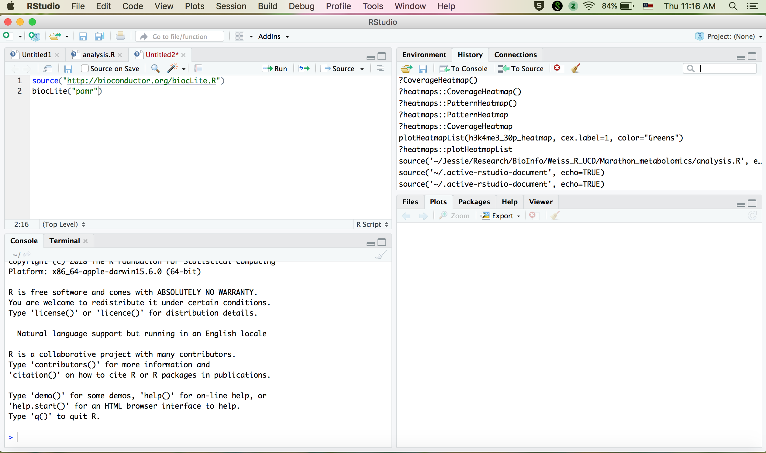
Scatter plot and line plot can be produced using the function plot().
x <- c(1:50)
y <- 1 + sqrt(x)/2
plot(x,y)
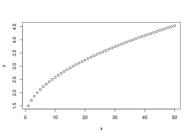
plot(x,y, type="l")
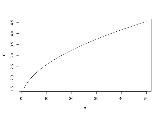
# plot both the points and lines
 first plot points
plot(x,y)
lines(x,y, type="l")
lines() can only be used to add information to a graph, while it cannot produce a graph on its own.
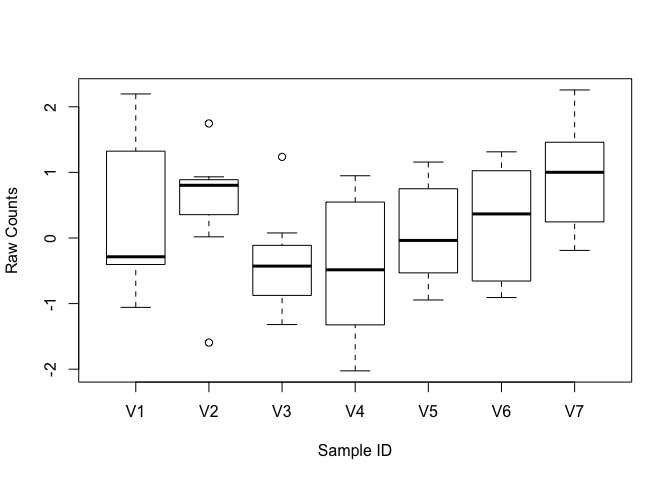
boxplot() can be used to summarize data.
boxplot(data, xlab="Sample ID", ylab="Raw Counts")
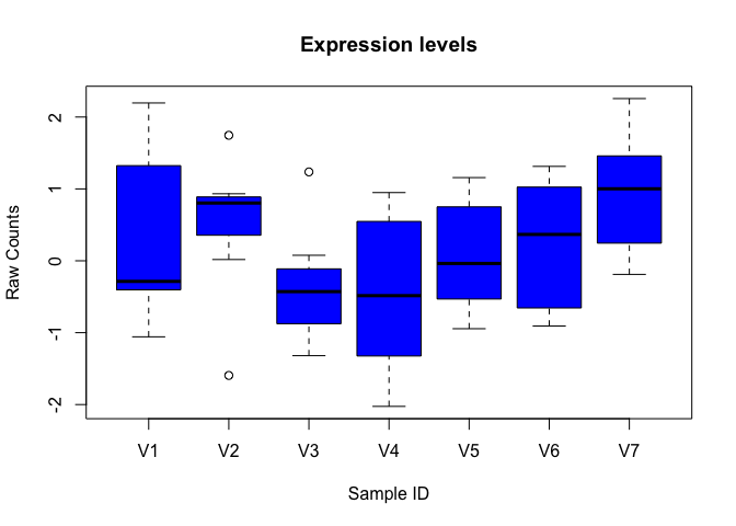
add more details to the plot.
boxplot(data, xlab="Sample ID", ylab="Raw Counts", main="Expression levels", col="blue", border="black")
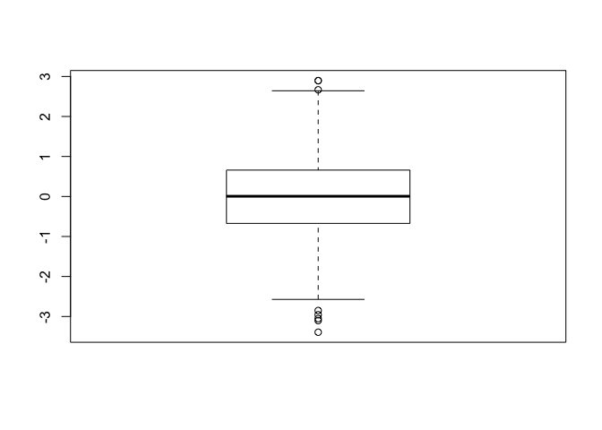
x <- rnorm(1000)
boxplot(x)
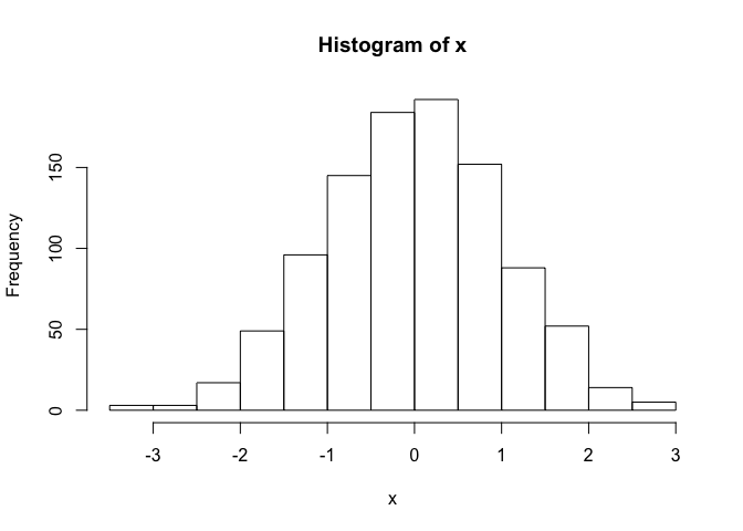
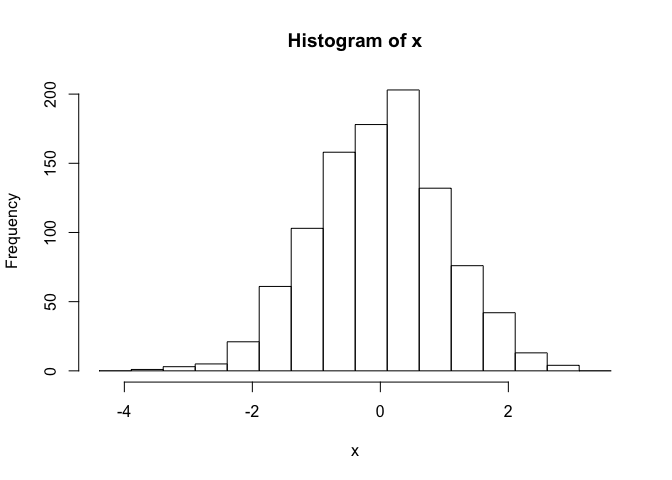
hist() can be used to create histograms of data.
hist(x)
# use user defined break points
hist(x, breaks=seq(range(x)[1]-1, range(x)[2]+1, by=0.5))
# clear plotting device/area
dev.off()
Topic 7. Install packages in R
Starting from Bioconductor version 3.8, the installation of packages is recommended to use BiocManager.
if (!requireNamespace("BiocManager"))
	install.packages("BiocManager")
 install core packages
BiocManager::install()
 install specific packages
BiocManager::install(c("ggplot2", "ShortRead"))
-
Bioconductor has a repository and release schedule that differ from R (Bioconductor has a ‘devel’ branch to which new packages and updates are introduced, and a stable ‘release’ branch emitted once every 6 months to which bug fixes but not new features are introduced). This mismatch causes that the version detected by install.packages() is sometimes not the most recent ‘release’.
-
A consequence of the distince ‘devel’ branch is that install.packages() sometimes points only to the ‘release’ repository, while users might want to have access to the leading-edge features in the develop version.
-
An indirect consequence of Bioconductor’s structured release is that packages generally have more extensive dependences with one another.
It is always recommended to update to the most current version of R and Bioconductor. If it is not possible and R < 3.5.0, please use the legacy approach to install Bioconductor packages
source("http://bioconductor.org/biocLite.R")
 install core packages
biocLite()
 install specific packages
biocLite("RCircos")
biocLite(c("IdeoViz", "devtools"))
The R function install.packages() can be used to install packages that are not part of Bioconductor.
install.packages("ggplot2", repos="http://cran.us.r-project.org")
Install from source of github.
library(devtools)
#install_github("stephenturner/qqman")
Topic 8. Save data in R session
To save history in R session
#savehistory(file="March27.history")

#loadhistory(file="March27.history")
To save objects in R session
save(list=c("x", "data"), file="March27.RData")

#load("March27.RData")
Challenge
Read in the reference fasta file for PhiX that you have downloaded this morning and find out the length of PhiX genome and GC content.
Hint: please look into bioconductor package ShortRead. The PhiX genome can be downloaded by following the instruction in Intro to Command-Line session. The link for the data is at ftp://igenome:G3nom3s4u@ussd-ftp.illumina.com/PhiX/Illumina/RTA/PhiX_Illumina_RTA.tar.gz