Single Cell Analysis with Seurat and some custom code!
Seurat is a popular R package that is designed for QC, analysis, and exploration of single cell data. Seurat aims to enable users to identify and interpret sources of heterogeneity from single cell transcriptomic measurements, and to integrate diverse types of single cell data. Further, the authors provide several tutorials on their website.
We start with loading needed libraries for R
library(Seurat)
library(tximport)
library(ggVennDiagram)
Load the Expression Matrix Data and create the combined base Seurat object.
Seurat provides a function Read10X to read in 10X data folder. First we read in data from each individual sample folder. Then, we initialize the Seurat object (CreateSeuratObject) with the raw (non-normalized data). Keep all genes expressed in >= 3 cells. Keep all cells with at least 200 detected genes. Also extracting sample names, calculating and adding in the metadata mitochondrial percentage of each cell. Some QA/QC Finally, saving the raw Seurat object.
A ens2sym.txt file
Reading in the salmon file, we will need to convert the ensembl ids to gene symbols. just like we did [here] (https://ucdavis-bioinformatics-training.github.io/2020-Advanced_Single_Cell_RNA_Seq/data_reduction/scMapping) to create the txp2gene.txt file from biomart, we will want to do the same for the ens2sym.txt file. You will need 3 columns “Gene stable ID”, “Gene stable ID version”, and “Gene name”. Your final file should look like this
Gene stable ID Gene stable ID version Gene name
ENSMUSG00000064372 ENSMUSG00000064372.1 mt-Tp
ENSMUSG00000064371 ENSMUSG00000064371.1 mt-Tt
ENSMUSG00000064370 ENSMUSG00000064370.1 mt-Cytb
ENSMUSG00000064369 ENSMUSG00000064369.1 mt-Te
ENSMUSG00000064368 ENSMUSG00000064368.1 mt-Nd6
ENSMUSG00000064367 ENSMUSG00000064367.1 mt-Nd5
ENSMUSG00000064366 ENSMUSG00000064366.1 mt-Tl2
ENSMUSG00000064365 ENSMUSG00000064365.1 mt-Ts2
ENSMUSG00000064364 ENSMUSG00000064364.1 mt-Th
ENSMUSG00000064363 ENSMUSG00000064363.1 mt-Nd4
ENSMUSG00000065947 ENSMUSG00000065947.3 mt-Nd4l
ENSMUSG00000064361 ENSMUSG00000064361.1 mt-Tr
ENSMUSG00000064360 ENSMUSG00000064360.1 mt-Nd3
## Cellranger
cellranger_orig <- Read10X_h5("Adv_comparison_outputs/654/outs/filtered_feature_bc_matrix.h5")
# If hdf5 isn't working read in from the mtx files
#cellranger_orig <- Read10X("Adv_comparison_outputs/654/outs/filtered_feature_bc_matrix")
s_cellranger_orig <- CreateSeuratObject(counts = cellranger_orig, min.cells = 3, min.features = 200, project = "cellranger")
s_cellranger_orig
An object of class Seurat
15203 features across 4907 samples within 1 assay
Active assay: RNA (15203 features, 0 variable features)
cellranger_htstream <- Read10X_h5("Adv_comparison_outputs/654_htstream/outs/filtered_feature_bc_matrix.h5")
s_cellranger_hts <- CreateSeuratObject(counts = cellranger_htstream, min.cells = 3, min.features = 200, project = "cellranger_hts")
s_cellranger_hts
An object of class Seurat
15197 features across 4918 samples within 1 assay
Active assay: RNA (15197 features, 0 variable features)
## STAR
star <- Read10X("Adv_comparison_outputs/654_htstream_star/outs/filtered_feature_bc_matrix")
s_star_hts <- CreateSeuratObject(counts = star, min.cells = 3, min.features = 200, project = "star")
s_star_hts
An object of class Seurat
15118 features across 4099 samples within 1 assay
Active assay: RNA (15118 features, 0 variable features)
## SALMON
txi <- tximport("Adv_comparison_outputs/654_htstream_salmon_decoys/alevin/quants_mat.gz", type="alevin")
importing alevin data is much faster after installing `fishpond` (>= 1.2.0)
reading in alevin gene-level counts across cells
## salmon is in ensembl IDs, need to convert to gene symbol
head(rownames(txi$counts))
[1] "ENSMUSG00000064370.1" "ENSMUSG00000064368.1" "ENSMUSG00000064367.1"
[4] "ENSMUSG00000064363.1" "ENSMUSG00000065947.3" "ENSMUSG00000064360.1"
ens2symbol <- read.table("ens2sym.txt",sep="\t",header=T,as.is=T)
map <- ens2symbol$Gene.name[match(rownames(txi$counts),ens2symbol$Gene.stable.ID.version)]

txi_counts <- txi$counts[-which(duplicated(map)),]
map <- map[-which(duplicated(map))]
rownames(txi_counts) <- map
dim(txi_counts)
[1] 35805 3919
s_salmon_hts <- CreateSeuratObject(counts = txi_counts , min.cells = 3, min.features = 200, project = "salmon")
s_salmon_hts
An object of class Seurat
15634 features across 3918 samples within 1 assay
Active assay: RNA (15634 features, 0 variable features)
# Need to Check Rows names/Col names before merge

# they however have different looking cell ids, need to fix
head(colnames(s_cellranger_orig))
[1] "AAACCTGAGATCACGG-1" "AAACCTGAGCATCATC-1" "AAACCTGAGCGCTCCA-1"
[4] "AAACCTGAGTGGGATC-1" "AAACCTGCAGACAGGT-1" "AAACCTGCATCATCCC-1"
head(colnames(s_star_hts))
[1] "AAACCTGAGATCACGG" "AAACCTGAGCATCATC" "AAACCTGAGCGCTCCA" "AAACCTGAGTGGGATC"
[5] "AAACCTGCAGACAGGT" "AAACCTGGTATAGGTA"
head(colnames(s_salmon_hts))
[1] "CGGACACCATTCACTT" "ACATACGAGAGTGAGA" "CTCACACAGAATTGTG" "CACACTCTCGGCCGAT"
[5] "CACAGGCCAATCTGCA" "TACTCATCATAGGATA"
s_cellranger_orig <- RenameCells(s_cellranger_orig, new.names = sapply(X = strsplit(colnames(s_cellranger_orig), split = "-"), FUN = "[", 1))

s_cellranger_hts <- RenameCells(s_cellranger_hts, new.names = sapply(X = strsplit(colnames(s_cellranger_hts), split = "-"), FUN = "[", 1))


## Merge the dataset
s_merged <- merge(s_cellranger_orig, y = c(s_cellranger_hts, s_star_hts, s_salmon_hts), add.cell.ids = c("cr.orig", "cr.hts", "star.hts", "salmon.hts"), project = "MapTest")
s_merged
An object of class Seurat
17597 features across 17842 samples within 1 assay
Active assay: RNA (17597 features, 0 variable features)
[1] "cr.orig_AAACCTGAGATCACGG" "cr.orig_AAACCTGAGCATCATC"
[3] "cr.orig_AAACCTGAGCGCTCCA" "cr.orig_AAACCTGAGTGGGATC"
[5] "cr.orig_AAACCTGCAGACAGGT" "cr.orig_AAACCTGCATCATCCC"
[1] "salmon.hts_TTGACTTAGCTTCGCG" "salmon.hts_AAAGTAGGTACGAAAT"
[3] "salmon.hts_CTTTGCGAGGCGTACA" "salmon.hts_ACACCAAGTGTGACCC"
[5] "salmon.hts_ACACTGATCGCCCTTA" "salmon.hts_ATCCGAAGTGCTGTAT"
table(s_merged$orig.ident)
cellranger cellranger_hts salmon star
4907 4918 3918 4099
table(table(sapply(X = strsplit(colnames(s_merged), split = "_"), FUN = "[", 2)))
1 2 3 4
55 719 411 3779
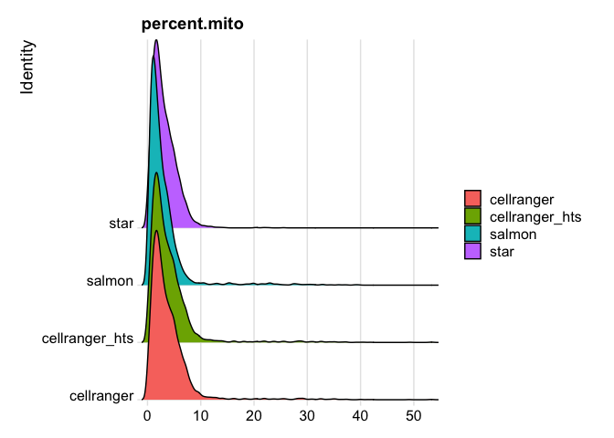
The percentage of reads that map to the mitochondrial genome
- Low-quality / dying cells often exhibit extensive mitochondrial content
- We calculate mitochondrial QC metrics with the PercentageFeatureSet function, which calculates the percentage of counts originating from a set of features.
- We use the set of all genes, in mouse these genes can be identified as those that begin with ‘mt’, in human data they begin with MT.
s_merged$percent.mito <- PercentageFeatureSet(s_merged, pattern = "^mt-")
Lets spend a little time getting to know the Seurat object.
The Seurat object is the center of each single cell analysis. It stores all information associated with the dataset, including data, annotations, analyses, etc. The R function slotNames can be used to view the slot names within an object.
[1] "assays" "meta.data" "active.assay" "active.ident" "graphs"
[6] "neighbors" "reductions" "project.name" "misc" "version"
[11] "commands" "tools"
orig.ident nCount_RNA nFeature_RNA percent.mito
cr.orig_AAACCTGAGATCACGG cellranger 2452 1326 7.4225122
cr.orig_AAACCTGAGCATCATC cellranger 2655 1329 0.8286252
cr.orig_AAACCTGAGCGCTCCA cellranger 2853 1529 3.7504381
cr.orig_AAACCTGAGTGGGATC cellranger 3636 1912 0.5500550
cr.orig_AAACCTGCAGACAGGT cellranger 1104 795 1.3586957
cr.orig_AAACCTGCATCATCCC cellranger 514 412 5.8365759
Question(s)
- What slots are empty, what slots have data?
- What columns are available in meta.data?
- Look up the help documentation for subset?
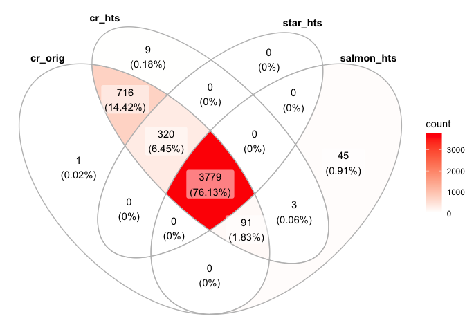
Now lets do some basic comparisons. Do they share the same cellbarcodes?
ggVennDiagram(list("cr_orig"=colnames(s_cellranger_orig),"cr_hts"=colnames(s_cellranger_hts), "star_hts"=colnames(s_star_hts), "salmon_hts"=colnames(s_salmon_hts)))
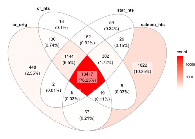
cr_orig_genes <- rowSums(as.matrix(GetAssayData(subset(s_merged, cells=colnames(s_merged)[s_merged$orig.ident=="cellranger"]))))
cr_hts_genes <- rowSums(as.matrix(GetAssayData(subset(s_merged, cells=colnames(s_merged)[s_merged$orig.ident=="cellranger_hts"]))))
star_hts_genes <- rowSums(as.matrix(GetAssayData(subset(s_merged, cells=colnames(s_merged)[s_merged$orig.ident=="star"]))))
salmon_hts_genes <- rowSums(as.matrix(GetAssayData(subset(s_merged, cells=colnames(s_merged)[s_merged$orig.ident=="salmon"]))))

minReads=0
ggVennDiagram(list("cr_orig"=names(cr_orig_genes[cr_orig_genes>minReads]),"cr_hts"=names(cr_hts_genes[cr_hts_genes>minReads]), "star_hts"=names(star_hts_genes[star_hts_genes>minReads]), "salmon_hts"=names(salmon_hts_genes[salmon_hts_genes>minReads])))
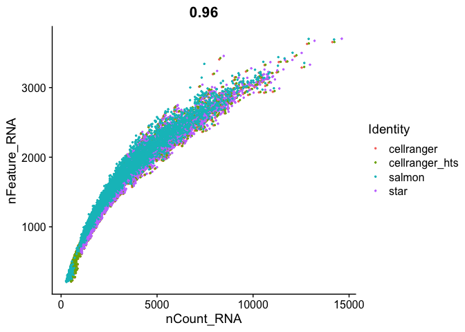
FeatureScatter(
  s_merged, "nCount_RNA", "nFeature_RNA",
  pt.size = 0.5)
Question(s)
- Spend a minute playing with minReads, see how the data changes.
- What are the sum of UMIs for each?
- Look up the help documentation for subset?
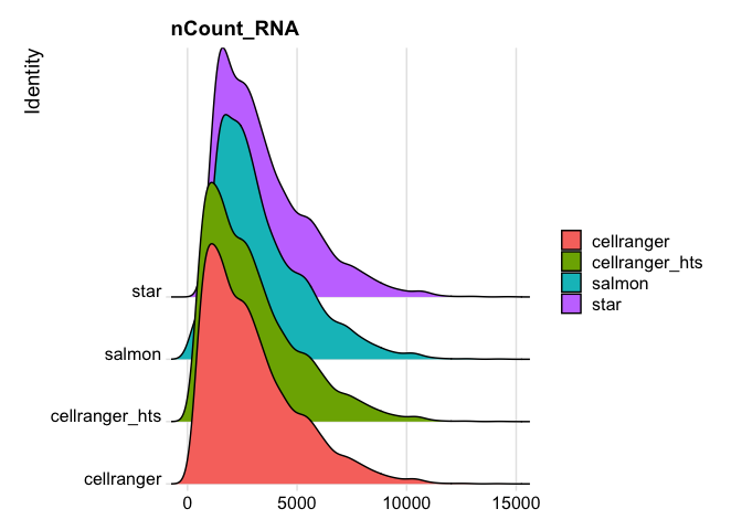
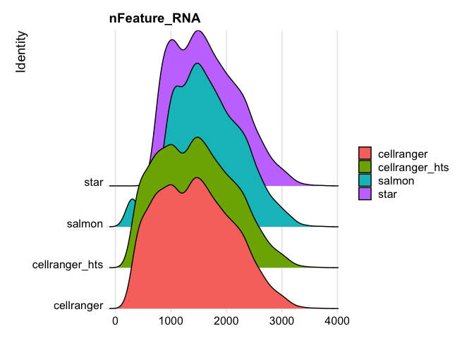
RidgePlot(s_merged, features="nCount_RNA")
Picking joint bandwidth of 335
RidgePlot(s_merged, features="nFeature_RNA")
Picking joint bandwidth of 105
RidgePlot(s_merged, features="percent.mito")
Picking joint bandwidth of 0.37
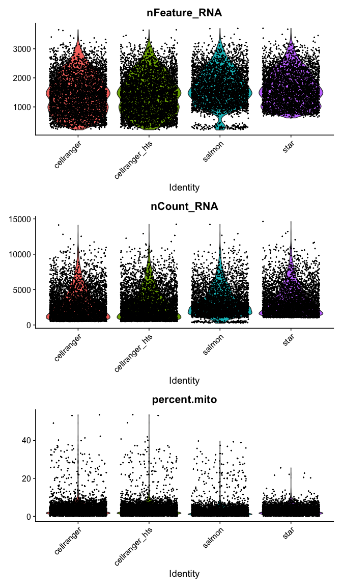
VlnPlot(
  s_merged,
  features = c("nFeature_RNA", "nCount_RNA","percent.mito"),
  ncol = 1, pt.size = 0.3)
s_merged <- NormalizeData(s_merged, normalization.method = "LogNormalize", scale.factor = 10000)
s_merged <- FindVariableFeatures(s_merged, selection.method = "vst", nfeatures = 2000)

all.genes <- rownames(s_merged)
s_merged <- ScaleData(s_merged, features = all.genes)
Centering and scaling data matrix
s_merged <- RunPCA(s_merged, features = VariableFeatures(object = s_merged))
PC_ 1
Positive: Adcyap1, Celf4, Gap43, Kit, Ngfr, Gal, Meg3, Fxyd7, Lynx1, Enah
Spock1, Pcp4, 6330403K07Rik, Mt1, Eno2, Syt2, Map2, Gpx3, Sv2b, S1pr3
Malat1, Fgf1, Dbpht2, Ptn, Cntn1, Scg2, Faim2, S100b, Npy1r, Stx1b
Negative: Sncg, Ubb, Txn1, Fxyd2, Atp6v0b, Lxn, Sh3bgrl3, Rabac1, Dctn3, Pfn1
Ppia, Fez1, Ndufa11, Cisd1, Ndufa4, Atp6v1f, Atpif1, S100a10, S100a6, Psmb2
Psmb6, Tmem45b, Prdx2, Elob, Nme1, Gabarapl2, Cox6a1, Bex2, Pop5, Bex3
PC_ 2
Positive: Cntn1, S100b, Nefh, Thy1, Cplx1, Tagln3, Hopx, Sv2b, Ntrk3, Lrrn1
Slc17a7, Nefm, Atp1b1, Atp2b2, Chchd10, Vsnl1, Nat8l, Nefl, Scn8a, Scn1a
Vamp1, Kcna2, Mcam, Scn1b, Endod1, Syt2, Lynx1, Sh3gl2, Scn4b, Cpne6
Negative: Cd24a, Malat1, Tmem233, Dusp26, Mal2, Prkca, Cd9, Osmr, Tmem158, Nppb
Carhsp1, Ift122, Cd44, Sst, Arpc1b, Calca, Npy2r, Gna14, Atpaf2, Gm525
Gadd45g, Tac1, Bhlhe41, Cd82, Adk, Meg3, Gng2, Nts, Scg2, Sntb1
PC_ 3
Positive: Gm28661, Gm10925, Rps7-ps3, Gm28437, Rpl10-ps3, Rpl9-ps6, Gm21981, Gm45234, Gm20390, Gm21988
Gm45713, Rps27rt, Gm10177, Gm10288, Gm10175, Uba52, Rnasek, Kxd1, Gm8430, Rpl10a-ps1
Nme2, Atp5o, Rpl17-ps3, Rps6-ps4, Gstp2, Gm12918, Gm29216, Rpl23a-ps3, Rpl27-ps3, Gm9843
Negative: Aldoa, Malat1, Atp5o.1, Meg3, Minos1, Usmg5, H2afz, 2010107E04Rik, Aes, Sept7
Atp5f1, Fam103a1, Tusc5, Fam96b, March2, 2410015M20Rik, Tmem55b, 1500011K16Rik, AC160336.1, Hist1h2bc
1110008F13Rik, H2afj, 3632451O06Rik, H2afy, Pqlc1, March6, Tmem55a, Sssca1, 1700020I14Rik, Fam19a4
PC_ 4
Positive: Tspan8, Jak1, Etv1, Resp18, Tmem233, Nppb, Adk, Sst, Skp1a, Scg2
Gm525, Osmr, Nts, Cystm1, Tesc, Npy2r, Nefh, Nsg1, S100b, Ift122
Map7d2, Thy1, Blvrb, Htr1f, Cd82, Prkca, Calm1, Ddah1, Atp1b1, Cysltr2
Negative: Gm7271, P2ry1, Rarres1, Th, Fxyd6, Tafa4, Wfdc2, Id4, Gfra2, Zfp521
Iqsec2, Rgs5, Rgs10, Tox3, Kcnd3, Cdkn1a, Rasgrp1, Alcam, Pou4f2, C1ql4
Rprm, Synpr, D130079A08Rik, Piezo2, Spink2, Ceacam10, Camk2n1, Bok, Grik1, Ptpre
PC_ 5
Positive: Basp1, Gm765, Prkar2b, Cd44, Rab27b, Calcb, Ctxn3, Lpar3, Ly86, Calca
Nefl, Aplp2, Mt3, Rgs7, Anks1b, Mrgprd, Nrn1l, Cd55, Nrn1, Gap43
Grik1, Serping1, Nmb, Klhl5, Rspo2, Spock3, Otoa, Ptprt, Synpr, S100a7l2
Negative: Nppb, Sst, Gm525, Nts, Osmr, Hpcal1, Npy2r, Htr1f, Jak1, Cysltr2
Ptprk, Tesc, Il31ra, Resp18, Tspan8, Blvrb, Cmtm7, Ada, Etv1, Fam178b
Cavin1, Camk2n1, Gstt2, Nbl1, Pde4c, Sntb1, Rarres1, Lgals1, Ddah1, Gm7271
use.pcs = 1:30
s_merged <- FindNeighbors(s_merged, dims = use.pcs)
Computing nearest neighbor graph
Computing SNN
s_merged <- FindClusters(s_merged, resolution = c(0.5,0.75,1.0))
Modularity Optimizer version 1.3.0 by Ludo Waltman and Nees Jan van Eck
Number of nodes: 17842
Number of edges: 691328
Running Louvain algorithm...
Maximum modularity in 10 random starts: 0.9579
Number of communities: 31
Elapsed time: 1 seconds
Modularity Optimizer version 1.3.0 by Ludo Waltman and Nees Jan van Eck
Number of nodes: 17842
Number of edges: 691328
Running Louvain algorithm...
Maximum modularity in 10 random starts: 0.9465
Number of communities: 33
Elapsed time: 1 seconds
Modularity Optimizer version 1.3.0 by Ludo Waltman and Nees Jan van Eck
Number of nodes: 17842
Number of edges: 691328
Running Louvain algorithm...
Maximum modularity in 10 random starts: 0.9364
Number of communities: 37
Elapsed time: 1 seconds
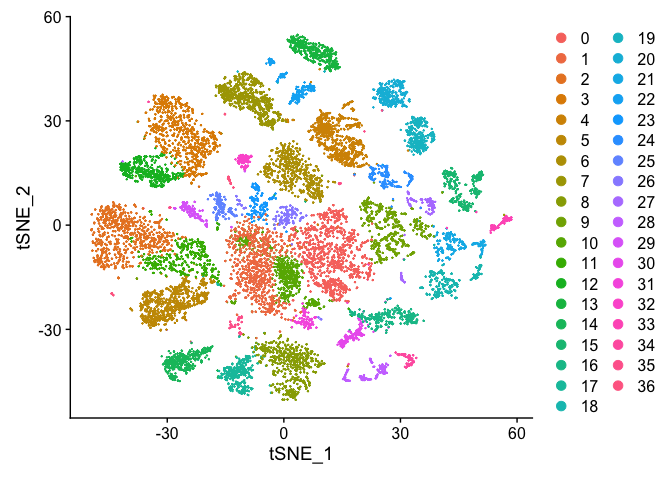
s_merged <- RunTSNE(s_merged, dims = use.pcs)
s_merged <- RunUMAP(s_merged, dims = use.pcs)
Warning: The default method for RunUMAP has changed from calling Python UMAP via reticulate to the R-native UWOT using the cosine metric
To use Python UMAP via reticulate, set umap.method to 'umap-learn' and metric to 'correlation'
This message will be shown once per session
19:04:18 UMAP embedding parameters a = 0.9922 b = 1.112
19:04:18 Read 17842 rows and found 30 numeric columns
19:04:18 Using Annoy for neighbor search, n_neighbors = 30
19:04:18 Building Annoy index with metric = cosine, n_trees = 50
0% 10 20 30 40 50 60 70 80 90 100%
[----|----|----|----|----|----|----|----|----|----|
**************************************************|
19:04:21 Writing NN index file to temp file /var/folders/74/h45z17f14l9g34tmffgq9nkw0000gn/T//RtmpI9wDI8/file1555f1d37fc
19:04:21 Searching Annoy index using 1 thread, search_k = 3000
19:04:25 Annoy recall = 100%
19:04:25 Commencing smooth kNN distance calibration using 1 thread
19:04:26 Initializing from normalized Laplacian + noise
19:04:27 Commencing optimization for 200 epochs, with 765114 positive edges
19:04:35 Optimization finished
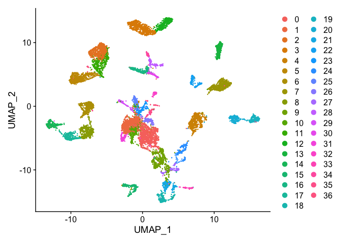
DimPlot(s_merged, reduction = "tsne")
DimPlot(s_merged, reduction = "umap")
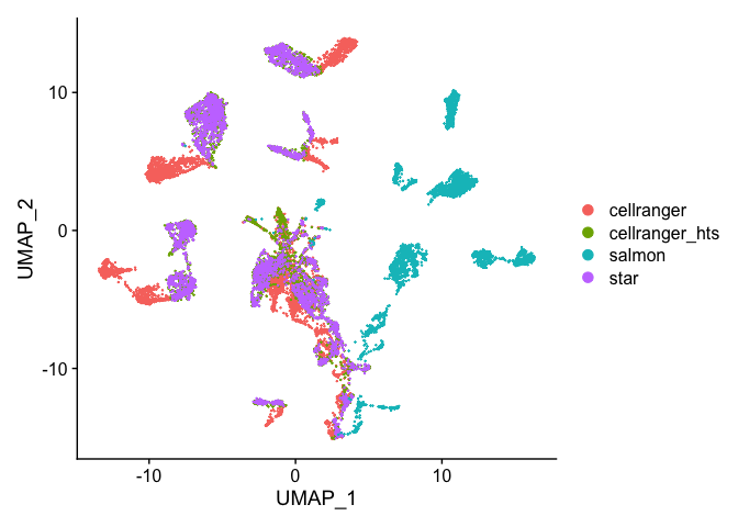
DimPlot(s_merged, group.by = "orig.ident", reduction = "umap")
Finally, save the original object, write out a tab-delimited table that could be read into excel, and view the object.
## Original dataset in Seurat class, with no filtering
save(s_merged,file="mapping_comparison_object.RData")
R version 4.0.0 (2020-04-24)
Platform: x86_64-apple-darwin17.0 (64-bit)
Running under: macOS Catalina 10.15.4
Matrix products: default
BLAS: /Library/Frameworks/R.framework/Versions/4.0/Resources/lib/libRblas.dylib
LAPACK: /Library/Frameworks/R.framework/Versions/4.0/Resources/lib/libRlapack.dylib
locale:
[1] en_US.UTF-8/en_US.UTF-8/en_US.UTF-8/C/en_US.UTF-8/en_US.UTF-8
attached base packages:
[1] stats graphics grDevices datasets utils methods base
other attached packages:
[1] ggVennDiagram_0.3 tximport_1.16.0 Seurat_3.1.5
loaded via a namespace (and not attached):
[1] nlme_3.1-148 tsne_0.1-3 sf_0.9-3
[4] bit64_0.9-7 RcppAnnoy_0.0.16 RColorBrewer_1.1-2
[7] httr_1.4.1 sctransform_0.2.1 tools_4.0.0
[10] R6_2.4.1 irlba_2.3.3 KernSmooth_2.23-17
[13] DBI_1.1.0 uwot_0.1.8 lazyeval_0.2.2
[16] colorspace_1.4-1 withr_2.2.0 tidyselect_1.1.0
[19] gridExtra_2.3 bit_1.1-15.2 compiler_4.0.0
[22] VennDiagram_1.6.20 formatR_1.7 hdf5r_1.3.2
[25] plotly_4.9.2.1 labeling_0.3 scales_1.1.1
[28] classInt_0.4-3 lmtest_0.9-37 ggridges_0.5.2
[31] pbapply_1.4-2 stringr_1.4.0 digest_0.6.25
[34] rmarkdown_2.1 pkgconfig_2.0.3 htmltools_0.4.0
[37] htmlwidgets_1.5.1 rlang_0.4.6 farver_2.0.3
[40] zoo_1.8-8 jsonlite_1.6.1 ica_1.0-2
[43] dplyr_0.8.5 magrittr_1.5 futile.logger_1.4.3
[46] patchwork_1.0.0 Matrix_1.2-18 Rcpp_1.0.4.6
[49] munsell_0.5.0 ape_5.3 reticulate_1.15
[52] lifecycle_0.2.0 stringi_1.4.6 yaml_2.2.1
[55] MASS_7.3-51.6 Rtsne_0.15 plyr_1.8.6
[58] grid_4.0.0 parallel_4.0.0 listenv_0.8.0
[61] ggrepel_0.8.2 crayon_1.3.4 lattice_0.20-41
[64] cowplot_1.0.0 splines_4.0.0 knitr_1.28
[67] pillar_1.4.4 igraph_1.2.5 future.apply_1.5.0
[70] reshape2_1.4.4 codetools_0.2-16 futile.options_1.0.1
[73] leiden_0.3.3 glue_1.4.1 evaluate_0.14
[76] lambda.r_1.2.4 data.table_1.12.8 renv_0.10.0
[79] BiocManager_1.30.10 png_0.1-7 vctrs_0.3.0
[82] gtable_0.3.0 RANN_2.6.1 purrr_0.3.4
[85] tidyr_1.1.0 future_1.17.0 assertthat_0.2.1
[88] ggplot2_3.3.0 xfun_0.14 rsvd_1.0.3
[91] RSpectra_0.16-0 e1071_1.7-3 class_7.3-17
[94] survival_3.1-12 viridisLite_0.3.0 tibble_3.0.1
[97] units_0.6-6 cluster_2.1.0 globals_0.12.5
[100] fitdistrplus_1.1-1 ellipsis_0.3.1 ROCR_1.0-11
