☰ Menu

      Advanced Single Cell RNA-Seq Workshop

Home
Introduction and Lectures
Intro to the Workshop and Core
Schedule
What is Bioinformatics/Genomics?
Experimental Design and Cost Estimation
Single Cell Sample Preparation - Dr. Diana Burkart-Waco
Support
Cheat Sheets
Software and Links
Scripts
Prerequisites
CLI - Logging in and Transferring Files
CLI - Intro to Command-Line
CLI - Advanced Command-Line (extra)
CLI - Running jobs on the Cluster and using modules
R - Getting Started
R - Intro to R
R - Prepare Data in R (extra)
R - Data in R (extra)
More Materials (extra)
Data Reduction
Generating Expression Matrices
Expression project setup
Preprocessing reads with HTStream
Generating Expression Tables
VDJ T cell and B cell
Velocity analysis
Data analysis
scRNA analysis prepare
Mapping Comparison
Anchoring (Comparison dataset)
Shiny App Install/Overview
App Practical Usage
AWS Hosted App (Optional)
Monocle
VDJ T cell and B cell analysis
Velocity analysis
ETC
Closing thoughts
Workshop Photos
Github page
Biocore website

In this section, we will learn how to take two separate datasets and “integrate” them, so that cells of the same type (across datasets) roughly fall into the same region of the tsne or umap plot (instead of separating by dataset first).

Integration is typically done in a few different scenarios, e.g.,

We start with loading needed libraries for R

library(Seurat)
library(tximport)
library(ggplot2)
library(ggVennDiagram)
library(cowplot)

Lets read the data back in and create a list of each dataset rather than merge like we did in Mapping_Comparisons

## Cellranger
cellranger_orig <- Read10X_h5("Adv_comparison_outputs/654/outs/filtered_feature_bc_matrix.h5")
# If hdf5 isn't working read in from the mtx files
#cellranger_orig <- Read10X("Adv_comparison_outputs/654/outs/filtered_feature_bc_matrix")
s_cellranger_orig <- CreateSeuratObject(counts = cellranger_orig, min.cells = 3, min.features = 200, project = "cellranger")
s_cellranger_orig
An object of class Seurat 15203 features across 4907 samples within 1 assay Active assay: RNA (15203 features, 0 variable features)
cellranger_htstream <- Read10X_h5("Adv_comparison_outputs/654_htstream/outs/filtered_feature_bc_matrix.h5")
s_cellranger_hts <- CreateSeuratObject(counts = cellranger_htstream, min.cells = 3, min.features = 200, project = "cellranger_hts")
s_cellranger_hts
An object of class Seurat 15197 features across 4918 samples within 1 assay Active assay: RNA (15197 features, 0 variable features)
## STAR
star <- Read10X("Adv_comparison_outputs/654_htstream_star/outs/filtered_feature_bc_matrix")
s_star_hts <- CreateSeuratObject(counts = star, min.cells = 3, min.features = 200, project = "star")
s_star_hts
An object of class Seurat 15118 features across 4099 samples within 1 assay Active assay: RNA (15118 features, 0 variable features)
## SALMON
txi <- tximport("Adv_comparison_outputs/654_htstream_salmon_decoys/alevin/quants_mat.gz", type="alevin")
importing alevin data is much faster after installing `fishpond` (>= 1.2.0)
reading in alevin gene-level counts across cells
## salmon is in ensembl IDs, need to convert to gene symbol
head(rownames(txi$counts))
[1] "ENSMUSG00000064370.1" "ENSMUSG00000064368.1" "ENSMUSG00000064367.1" [4] "ENSMUSG00000064363.1" "ENSMUSG00000065947.3" "ENSMUSG00000064360.1"
ens2symbol <- read.table("ens2sym.txt",sep="\t",header=T,as.is=T)
map <- ens2symbol$Gene.name[match(rownames(txi$counts),ens2symbol$Gene.stable.ID.version)]

txi_counts <- txi$counts[-which(duplicated(map)),]
map <- map[-which(duplicated(map))]
rownames(txi_counts) <- map
dim(txi_counts)
[1] 35805 3919
s_salmon_hts <- CreateSeuratObject(counts = txi_counts , min.cells = 3, min.features = 200, project = "salmon")
s_salmon_hts
An object of class Seurat 15634 features across 3918 samples within 1 assay Active assay: RNA (15634 features, 0 variable features)
# Need to Check Col names before merge 

# they however have different looking cell ids, need to fix
head(colnames(s_cellranger_orig))
[1] "AAACCTGAGATCACGG-1" "AAACCTGAGCATCATC-1" "AAACCTGAGCGCTCCA-1" [4] "AAACCTGAGTGGGATC-1" "AAACCTGCAGACAGGT-1" "AAACCTGCATCATCCC-1"
head(colnames(s_star_hts))
[1] "AAACCTGAGATCACGG" "AAACCTGAGCATCATC" "AAACCTGAGCGCTCCA" "AAACCTGAGTGGGATC" [5] "AAACCTGCAGACAGGT" "AAACCTGGTATAGGTA"
head(colnames(s_salmon_hts))
[1] "CGGACACCATTCACTT" "ACATACGAGAGTGAGA" "CTCACACAGAATTGTG" "CACACTCTCGGCCGAT" [5] "CACAGGCCAATCTGCA" "TACTCATCATAGGATA"
s_cellranger_orig <- RenameCells(s_cellranger_orig, new.names = sapply(X = strsplit(colnames(s_cellranger_orig), split = "-"), FUN = "[", 1))

s_cellranger_hts <- RenameCells(s_cellranger_hts, new.names = sapply(X = strsplit(colnames(s_cellranger_hts), split = "-"), FUN = "[", 1))

Instead of merging the datasets (column binding the cells). This time we are going to make an R list

s_list = list(s_cellranger_orig, s_cellranger_hts, s_star_hts, s_salmon_hts)

using the Standare Seurat technique

Normalization and Variable Features

Before we identify integration sites and find anchors, First perform normalzation and identify variable features for each

s_standard = s_list
for (i in 1:length(s_standard)) {
    s_standard[[i]] <- NormalizeData(s_standard[[i]], verbose = FALSE)
    s_standard[[i]] <- FindVariableFeatures(s_standard[[i]], selection.method = "vst", nfeatures = 2000, verbose = FALSE)
}

Identify “anchors”

Next, we identify anchors using the FindIntegrationAnchors function, which takes a list of Seurat objects as input.

?FindIntegrationAnchors

We use all default parameters here for identifying anchors, including the ‘dimensionality’ of the dataset (30)

s.anchors_standard <- FindIntegrationAnchors(object.list = s_standard, dims = 1:30)
Warning in CheckDuplicateCellNames(object.list = object.list): Some cell names are duplicated across objects provided. Renaming to enforce unique cell names.
Computing 2000 integration features
Scaling features for provided objects
Finding all pairwise anchors
Running CCA
Merging objects
Finding neighborhoods
Finding anchors
Found 13730 anchors
Filtering anchors
Retained 10677 anchors
Extracting within-dataset neighbors
Running CCA
Merging objects
Finding neighborhoods
Finding anchors
Found 12422 anchors
Filtering anchors
Retained 9785 anchors
Extracting within-dataset neighbors
Running CCA
Merging objects
Finding neighborhoods
Finding anchors
Found 12447 anchors
Filtering anchors
Retained 9857 anchors
Extracting within-dataset neighbors
Running CCA
Merging objects
Finding neighborhoods
Finding anchors
Found 11951 anchors
Filtering anchors
Retained 9582 anchors
Extracting within-dataset neighbors
Running CCA
Merging objects
Finding neighborhoods
Finding anchors
Found 11865 anchors
Filtering anchors
Retained 9548 anchors
Extracting within-dataset neighbors
Running CCA
Merging objects
Finding neighborhoods
Finding anchors
Found 11628 anchors
Filtering anchors
Retained 9192 anchors
Extracting within-dataset neighbors
s.integrated_standard <- IntegrateData(anchorset = s.anchors_standard, dims = 1:30)
Merging dataset 4 into 1
Extracting anchors for merged samples
Finding integration vectors
Finding integration vector weights
Integrating data
Merging dataset 3 into 2
Extracting anchors for merged samples
Finding integration vectors
Finding integration vector weights
Integrating data
Merging dataset 1 4 into 2 3
Extracting anchors for merged samples
Finding integration vectors
Finding integration vector weights
Integrating data
Warning: Adding a command log without an assay associated with it

The returned object

will contain a new Assay, which holds an integrated (or ‘batch-corrected’) expression matrix for all cells, enabling them to be jointly analyzed.

s.integrated_standard
An object of class Seurat 19597 features across 17842 samples within 2 assays Active assay: integrated (2000 features, 2000 variable features) 1 other assay present: RNA
DefaultAssay(object = s.integrated_standard) <- "RNA"
s.integrated_standard
An object of class Seurat 19597 features across 17842 samples within 2 assays Active assay: RNA (17597 features, 0 variable features) 1 other assay present: integrated
DefaultAssay(object = s.integrated_standard) <- "integrated"
s.integrated_standard
An object of class Seurat 19597 features across 17842 samples within 2 assays Active assay: integrated (2000 features, 2000 variable features) 1 other assay present: RNA

Now visualize after anchoring and integration

Run the standard workflow for visualization and clustering

s.integrated_standard <- ScaleData(s.integrated_standard, verbose = FALSE)
s.integrated_standard <- RunPCA(s.integrated_standard, npcs = 30, verbose = FALSE)
s.integrated_standard <- RunUMAP(s.integrated_standard, reduction = "pca", dims = 1:30)
Warning: The default method for RunUMAP has changed from calling Python UMAP via reticulate to the R-native UWOT using the cosine metric To use Python UMAP via reticulate, set umap.method to 'umap-learn' and metric to 'correlation' This message will be shown once per session
07:27:59 UMAP embedding parameters a = 0.9922 b = 1.112
07:27:59 Read 17842 rows and found 30 numeric columns
07:27:59 Using Annoy for neighbor search, n_neighbors = 30
07:27:59 Building Annoy index with metric = cosine, n_trees = 50
0% 10 20 30 40 50 60 70 80 90 100%
[----|----|----|----|----|----|----|----|----|----|
**************************************************| 07:28:02 Writing NN index file to temp file /var/folders/74/h45z17f14l9g34tmffgq9nkw0000gn/T//RtmpjoDPLs/file172534f1f53cb 07:28:02 Searching Annoy index using 1 thread, search_k = 3000 07:28:08 Annoy recall = 100% 07:28:08 Commencing smooth kNN distance calibration using 1 thread 07:28:09 Initializing from normalized Laplacian + noise 07:28:11 Commencing optimization for 200 epochs, with 795910 positive edges 07:28:19 Optimization finished
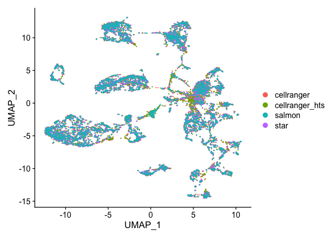
DimPlot(s.integrated_standard, reduction = "umap")

Excersise

Check the help of FindIntegrationAnchors. What happens when you change dims (try varying this parameter over a broad range, for example between 10 and 50), k.anchor, k.filter and k.score?

dims Which dimensions to use from the CCA to specify the neighbor search space
k.anchor How many neighbors (k) to use when picking anchors
k.filter How many neighbors (k) to use when filtering anchors
k.score How many neighbors (k) to use when scoring anchors

Example

s.anchors_standard <- FindIntegrationAnchors(object.list = s_standard, dims = 1:2)

Now lets look closer

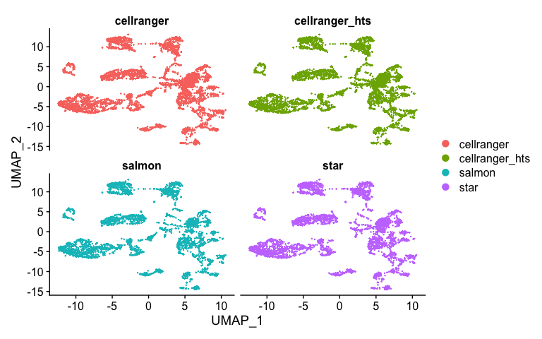
Splitting by prepocessing type

DimPlot(s.integrated_standard, reduction = "umap", split.by = "orig.ident", ncol=2)

We can conduct more analysis, perform clustering

s.integrated_standard <- FindNeighbors(s.integrated_standard, reduction = "pca", dims = 1:30)
Computing nearest neighbor graph
Computing SNN
s.integrated_standard <- FindClusters(s.integrated_standard, resolution = 0.5)
Modularity Optimizer version 1.3.0 by Ludo Waltman and Nees Jan van Eck Number of nodes: 17842 Number of edges: 761977 Running Louvain algorithm... Maximum modularity in 10 random starts: 0.9468 Number of communities: 25 Elapsed time: 2 seconds
p1 <- DimPlot(s.integrated_standard, reduction = "umap", group.by = "orig.ident")
p2 <- DimPlot(s.integrated_standard, reduction = "umap", label = TRUE, label.size = 6)
Warning: Using `as.character()` on a quosure is deprecated as of rlang 0.3.0. Please use `as_label()` or `as_name()` instead. This warning is displayed once per session.
plot_grid(p1, p2)

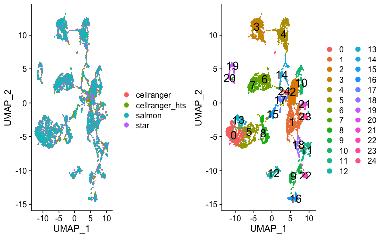
Now lets look at cluster representation per dataset

t <- table(s.integrated_standard$integrated_snn_res.0.5, s.integrated_standard$orig.ident)
t
cellranger cellranger_hts salmon star 0 430 431 430 430 1 446 451 361 395 2 527 535 245 335 3 426 428 379 398 4 407 405 348 367 5 338 336 279 294 6 325 325 261 287 7 224 224 217 220 8 202 203 181 187 9 166 167 119 135 10 158 160 119 132 11 148 149 119 131 12 141 142 121 131 13 107 107 104 106 14 142 141 51 49 15 122 126 127 3 16 102 101 80 90 17 111 110 54 66 18 77 76 70 75 19 55 55 51 51 20 52 52 51 53 21 63 59 38 43 22 51 51 48 50 23 50 47 46 48 24 37 37 19 23
round(sweep(t,MARGIN=2, STATS=colSums(t), FUN = "/")*100,1)
cellranger cellranger_hts salmon star 0 8.8 8.8 11.0 10.5 1 9.1 9.2 9.2 9.6 2 10.7 10.9 6.3 8.2 3 8.7 8.7 9.7 9.7 4 8.3 8.2 8.9 9.0 5 6.9 6.8 7.1 7.2 6 6.6 6.6 6.7 7.0 7 4.6 4.6 5.5 5.4 8 4.1 4.1 4.6 4.6 9 3.4 3.4 3.0 3.3 10 3.2 3.3 3.0 3.2 11 3.0 3.0 3.0 3.2 12 2.9 2.9 3.1 3.2 13 2.2 2.2 2.7 2.6 14 2.9 2.9 1.3 1.2 15 2.5 2.6 3.2 0.1 16 2.1 2.1 2.0 2.2 17 2.3 2.2 1.4 1.6 18 1.6 1.5 1.8 1.8 19 1.1 1.1 1.3 1.2 20 1.1 1.1 1.3 1.3 21 1.3 1.2 1.0 1.0 22 1.0 1.0 1.2 1.2 23 1.0 1.0 1.2 1.2 24 0.8 0.8 0.5 0.6

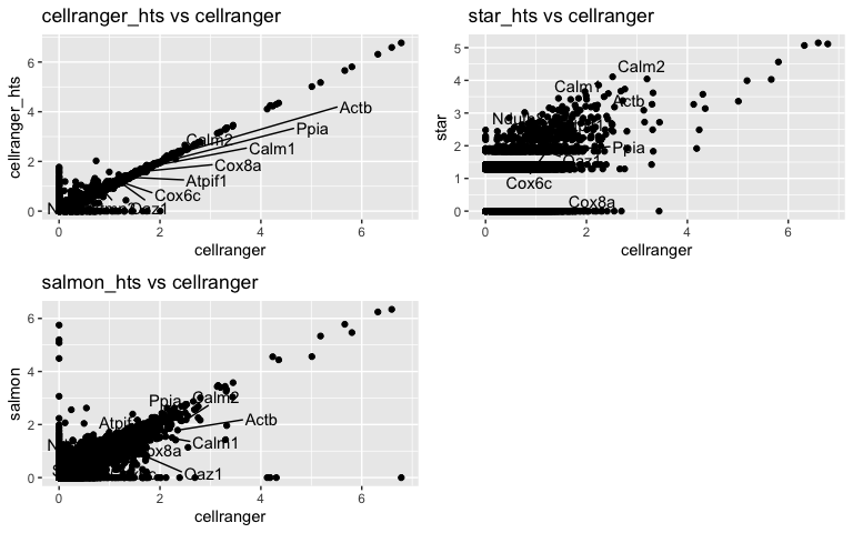
Lets Zero in on cluster 15 some more

markers = FindMarkers(s.integrated_standard, ident.1="15")
top10 <- rownames(markers)[1:10]
head(markers)
p_val avg_logFC pct.1 pct.2 p_val_adj Calm1 1.926295e-180 -1.889314 0.550 0.984 3.852590e-177 Cox8a 3.445073e-164 -1.700591 0.444 0.969 6.890145e-161 Ppia 1.860959e-161 -1.804402 0.648 0.980 3.721918e-158 Cox6c 1.457237e-152 -1.679867 0.323 0.935 2.914474e-149 Actb 7.767536e-152 -1.964185 0.624 0.991 1.553507e-148 Stmn3 1.262762e-151 -1.806284 0.468 0.922 2.525524e-148
cluster15 <- subset(s.integrated_standard, idents = "15")
Idents(cluster15) <- "orig.ident"
avg.cell.exp <- log1p(AverageExpression(cluster15, verbose = FALSE)$RNA)
avg.cell.exp$gene <- rownames(avg.cell.exp)

head(avg.cell.exp)
cellranger cellranger_hts star salmon gene Xkr4 0.0000000 0.00000000 0.000000 0.0000000 Xkr4 Sox17 0.1443089 0.13880722 0.000000 0.1805196 Sox17 Mrpl15 0.0000000 0.00000000 0.000000 0.0000000 Mrpl15 Lypla1 0.5149806 0.50052080 1.280963 0.5133444 Lypla1 Tcea1 0.1020398 0.09822009 0.000000 0.3844843 Tcea1 Rgs20 0.0000000 0.00000000 0.000000 0.0000000 Rgs20
p1 <- ggplot(avg.cell.exp, aes(cellranger, cellranger_hts)) + geom_point() + ggtitle("cellranger_hts vs cellranger")
p1 <- LabelPoints(plot = p1, points = top10, repel = TRUE)
When using repel, set xnudge and ynudge to 0 for optimal results
p2 <- ggplot(avg.cell.exp, aes(cellranger, star)) + geom_point() + ggtitle("star_hts vs cellranger")
p2 <- LabelPoints(plot = p2, points = top10, repel = TRUE)
When using repel, set xnudge and ynudge to 0 for optimal results
p3 <- ggplot(avg.cell.exp, aes(cellranger, salmon)) + geom_point() + ggtitle("salmon_hts vs cellranger")
p3 <- LabelPoints(plot = p3, points = top10, repel = TRUE)
When using repel, set xnudge and ynudge to 0 for optimal results
plot_grid(p1,p2,p3, ncol = 2)

Possible continued analysis

We know the majority of ‘cells’ are in common between the datasets, so how is the cell barcode representation in each cluster. So for this cluster 15, what is the overlap in cells for cellranger/salmon/star if those cells are present in star, where did they go? Which cluster can they be found in.

How I would go about doing this Get the superset of cell barcode from all 4 methods for cluster 15. Then extract these cells from the whole dataset (subset) and table the occurace of this subset of cells [superset of those found in 15], sample by cluster like we did above.

ALSO

Salmon had a few ‘unique’ cells, where did these go?

More reading

For a larger list of alignment methods, as well as an evaluation of them, see Gerald Quons paper, “scAlign: a tool for alignment, integration, and rare cell identification from scRNA-seq data”

Using SCTransform (Not Evaluated because it takes a really long time)

s_sct <- s_list
for (i in 1:length(s_sct)) {
    s_sct[[i]] <- SCTransform(s_sct[[i]], verbose = FALSE)
}
s_features_sct <- SelectIntegrationFeatures(object.list = s_sct, nfeatures = 2000)

s_sct <- PrepSCTIntegration(object.list = s_sct, anchor.features = s_features, 
    verbose = FALSE)

Identify anchors and integrate the datasets.

Commands are identical to the standard workflow, but make sure to set normalization.method = ‘SCT’:

s_anchors_sct <- FindIntegrationAnchors(object.list = s_sct, normalization.method = "SCT",  anchor.features = s_features, verbose = FALSE)
s_integrated_sct <- IntegrateData(anchorset = s_anchors_sct, normalization.method = "SCT", verbose = FALSE)

Now visualize after anchoring and integration

However, do not sun ScaleData, SCTransform does this step

s.integrated_sct <- RunPCA(s.integrated_sct, npcs = 30, verbose = FALSE)
s.integrated_sct <- RunUMAP(s.integrated_sct, reduction = "pca", dims = 1:30)
DimPlot(s.integrated_sct, reduction = "umap")

Rest is the same

More reading on SCTransform

Normalization and variance stabilization of single-cell RNA-seq data using regularized negative binomial regression

Finally, save the original object, write out a tab-delimited table that could be read into excel, and view the object.

## anchored dataset in Seurat class
save(s.integrated_standard,file="anchored_object.RData")

Session Information

sessionInfo()
R version 4.0.0 (2020-04-24) Platform: x86_64-apple-darwin17.0 (64-bit) Running under: macOS Catalina 10.15.4 Matrix products: default BLAS: /Library/Frameworks/R.framework/Versions/4.0/Resources/lib/libRblas.dylib LAPACK: /Library/Frameworks/R.framework/Versions/4.0/Resources/lib/libRlapack.dylib locale: [1] en_US.UTF-8/en_US.UTF-8/en_US.UTF-8/C/en_US.UTF-8/en_US.UTF-8 attached base packages: [1] stats graphics grDevices datasets utils methods base other attached packages: [1] cowplot_1.0.0 ggVennDiagram_0.3 ggplot2_3.3.0 tximport_1.16.0 [5] Seurat_3.1.5 loaded via a namespace (and not attached): [1] nlme_3.1-148 tsne_0.1-3 sf_0.9-3 [4] bit64_0.9-7 RcppAnnoy_0.0.16 RColorBrewer_1.1-2 [7] httr_1.4.1 sctransform_0.2.1 tools_4.0.0 [10] R6_2.4.1 irlba_2.3.3 KernSmooth_2.23-17 [13] DBI_1.1.0 uwot_0.1.8 lazyeval_0.2.2 [16] colorspace_1.4-1 withr_2.2.0 tidyselect_1.1.0 [19] gridExtra_2.3 bit_1.1-15.2 compiler_4.0.0 [22] VennDiagram_1.6.20 formatR_1.7 hdf5r_1.3.2 [25] plotly_4.9.2.1 labeling_0.3 scales_1.1.1 [28] classInt_0.4-3 lmtest_0.9-37 ggridges_0.5.2 [31] pbapply_1.4-2 stringr_1.4.0 digest_0.6.25 [34] rmarkdown_2.1 pkgconfig_2.0.3 htmltools_0.4.0 [37] limma_3.44.1 htmlwidgets_1.5.1 rlang_0.4.6 [40] farver_2.0.3 zoo_1.8-8 jsonlite_1.6.1 [43] ica_1.0-2 dplyr_0.8.5 magrittr_1.5 [46] futile.logger_1.4.3 patchwork_1.0.0 Matrix_1.2-18 [49] Rcpp_1.0.4.6 munsell_0.5.0 ape_5.3 [52] reticulate_1.15 lifecycle_0.2.0 stringi_1.4.6 [55] yaml_2.2.1 MASS_7.3-51.6 Rtsne_0.15 [58] plyr_1.8.6 grid_4.0.0 parallel_4.0.0 [61] listenv_0.8.0 ggrepel_0.8.2 crayon_1.3.4 [64] lattice_0.20-41 splines_4.0.0 knitr_1.28 [67] pillar_1.4.4 igraph_1.2.5 future.apply_1.5.0 [70] reshape2_1.4.4 codetools_0.2-16 futile.options_1.0.1 [73] leiden_0.3.3 glue_1.4.1 evaluate_0.14 [76] lambda.r_1.2.4 data.table_1.12.8 renv_0.10.0 [79] BiocManager_1.30.10 png_0.1-7 vctrs_0.3.0 [82] gtable_0.3.0 RANN_2.6.1 purrr_0.3.4 [85] tidyr_1.1.0 future_1.17.0 assertthat_0.2.1 [88] xfun_0.14 rsvd_1.0.3 RSpectra_0.16-0 [91] e1071_1.7-3 class_7.3-17 survival_3.1-12 [94] viridisLite_0.3.0 tibble_3.0.1 units_0.6-6 [97] cluster_2.1.0 globals_0.12.5 fitdistrplus_1.1-1 [100] ellipsis_0.3.1 ROCR_1.0-11