Generating a Single Cell Gene Expression Matrix
Most analyses have two stages: data reduction and biological analysis. Statistical analyses of scRNA-seq data take as their starting point an expression matrix, where each row represents a gene and each column represents a sample (in scRNAseq a cell). Each entry in the matrix represents the number of reads (expression level) of a particular gene in a given sample (cell). In most cases the number of unique reads (post umi filtering) assigned to that gene in that sample/cell. Generating the expression matrix often involves some, or all, of the following.

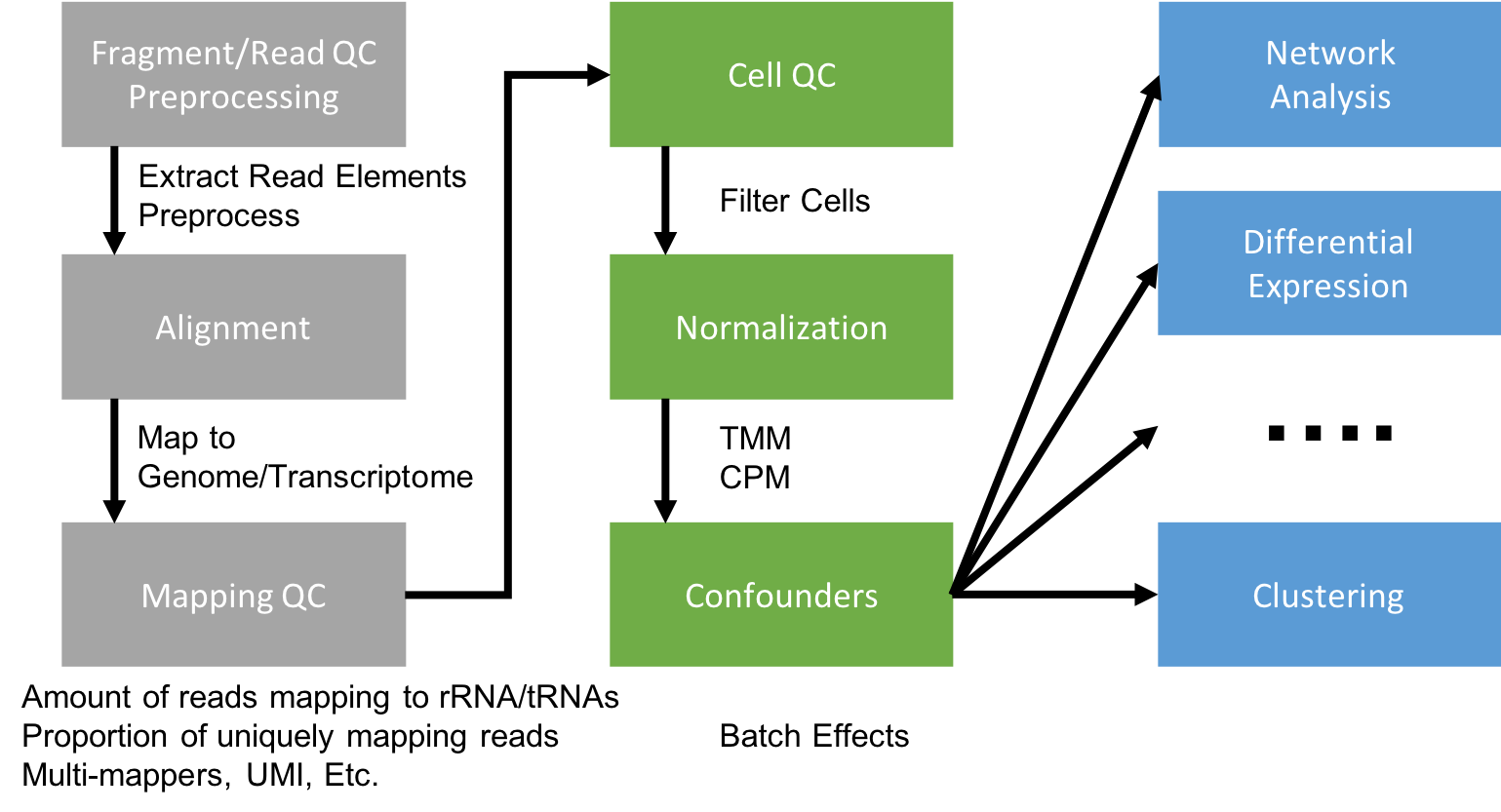
Flowchart of scRNAseq analysis
Preprocessing and mapping reads
Raw fastq files first need to be preprocessed, extracting any elements that are a part of the sequence read.
- Library Barcode (library Index) - Used to pool multiple libraries on one sequencing lane
- Cell Barcode – Used to identify the cell the read came from
- Unique Molecular Index (UMI) – Used to identify reads that arise during PCR duplication
- RNA Transcript Read – Used to identify the gene a read came from
The remaining sequences are mapped to a reference.
For 10X genomics datasets, there is the cellranger application. If you’d rather not use cellranger, or have non-10X data there is also STAR solo aligner. For large full-transcript datasets from well annotated organisms (e.g. mouse, human) pseudo-alignment method Salmon is also a good choice for alignment. For full-length datasets with tens- or hundreds of thousands of reads per cell pseudo-aligners become more appealing since their run-time can be several orders of magnitude less than traditional aligners.
Note, if spike-ins are used, the spike-in sequences should be added to the reference sequence prior to mapping.
Gene Counting
Cellranger, STAR solo, and Salmon Alevin all quantify the expression level of each gene for each cell taking into account UMI sequence as a part of its output.
Specific steps to be performed are dependent on the type of library, the element layout of the read, and the sequencing parameters.
scRNAseq Libraries
Generating scRNAseq libraries is currently an active area of research with several protocols being published in the last few years, including:
- CEL-seq Hashimshony, 2012
- CEL-seq2 Hashimshony, 2016
- DroNC-seq Habib, 2017
- Drop-seq Macosko, 2015
- InDrop-seq Klein, 2015
- MATQ-seq Sheng, 2017_2018
- MARS-seq Jaitin, 2014
- SCRB-seq Soumillon, 2014
- Seq-well Gierahn, 2017
- Smart-seq Picelli, 2014
- Smart-seq2 Picelli, 2014
- SMARTer clontech
- STRT-seq Islam, 2014
- 3’ UPX Qiagen
Differences between the methods are are in how they capture and quantify gene expression (either full-length or tag-based).
Full-length capture tries to achieve a uniform coverage of each transcript (many reads per transcript). Tag-based protocols only capture either the 5’- or 3’-end of each tran script (single read per transcript). Choice in method determines what types of analyses the data can be used for. Full-length capture can be used to distinguish different iso-forms, where tag-based method is best used for only gene abundance.
- Tag-based 3’ counting techniques
- 1 read per transcript
- Based on polyA
- Expression analysis only
- Fewer reads per cell needed needed
- Less noise in expression patterns
- Full-length
- Based on polyA
- Expression analysis
- Splicing information
- The more information desired beyond expression, the higher the reads needed per cell
Regardless of the protocol, you should spend some time to understand the structure of the read after library preparation.

Elements to a 10x read (V3)
Packages for downstream analysis
There are many and more being developed. For smaller experiments < 5000 cells, the R packages SingleCellExperiment, scater, SC3 are good choices. For larger experiments (> 5000 cells), the R package Seurat offers a complete solution.
A nice page keeping track of single-cell software can be found here.
