
Load libraries
library(Seurat)
Load the Seurat object
load(file="pre_sample_corrected.RData")
experiment.aggregate
An object of class Seurat
12811 features across 2681 samples within 1 assay
Active assay: RNA (12811 features)
experiment.test <- experiment.aggregate
set.seed(12345)
rand.genes <- sample(1:nrow(experiment.test), 500,replace = F)
mat <- as.matrix(GetAssayData(experiment.test, slot="data"))
mat[rand.genes,experiment.test$batchid=="Batch2"] <- mat[rand.genes,experiment.test$batchid=="Batch2"] + 0.18
experiment.test = SetAssayData(experiment.test, slot="data", new.data= mat )
Exploring Batch effects 3 ways, none, Seurat [vars.to.regress] and COMBAT
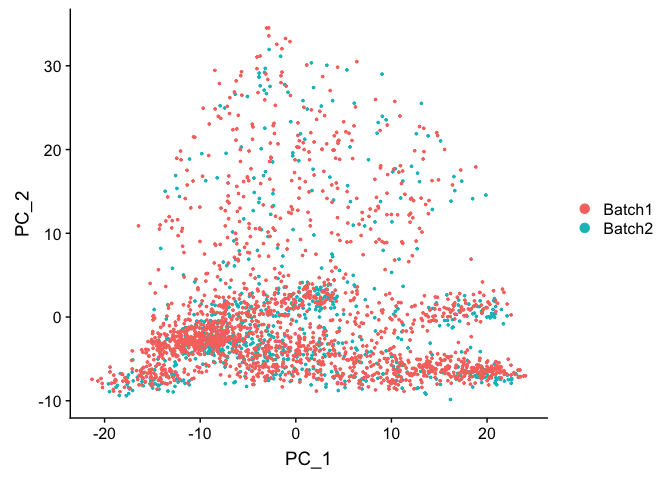
First lets view the data without any corrections
PCA in prep for tSNE
ScaleData - Scales and centers genes in the dataset.
?ScaleData
experiment.test.noc <- ScaleData(object = experiment.test)
Centering and scaling data matrix
Run PCA
experiment.test.noc <- RunPCA(object = experiment.test.noc)
PC_ 1
Positive: Txn1, Sncg, Fez1, S100a10, Atp6v0b, Lxn, Dctn3, Tppp3, Sh3bgrl3, Rabac1
Cisd1, Ppia, Fxyd2, Stmn3, Atp6v1f, Ndufa11, Atp5g1, Bex2, Atpif1, Uchl1
Ndufa4, Psmb6, Ubb, Hagh, Anxa2, Gabarapl2, Rgs10, Nme1, Prdx2, Psmb3
Negative: Mt1, Malat1, Adcyap1, Ptn, Apoe, Zeb2, Mt2, Timp3, Fabp7, Gpm6b
Gal, Kit, Qk, Plp1, Atp2b4, Ifitm3, 6330403K07Rik, Sparc, Id3, Gap43
Selenop, Gpx3, Rgcc, Zfp36l1, Scg2, Cbfb, Zfp36, Igfbp7, Marcksl1, Phlda1
PC_ 2
Positive: Nefh, Cntn1, Thy1, S100b, Sv2b, Cplx1, Slc17a7, Vamp1, Nefm, Lynx1
Endod1, Scn1a, Atp1b1, Vsnl1, Nat8l, Ntrk3, Sh3gl2, Fam19a2, Eno2, Scn1b
Spock1, Scn8a, Glrb, Syt2, Lrrn1, Scn4b, Lgi3, Atp2b2, Snap25, Cpne6
Negative: Malat1, Cd24a, Tmem233, Cd9, Dusp26, Mal2, Carhsp1, Tmem158, Fxyd2, Ctxn3
Ubb, Arpc1b, Crip2, Prkca, S100a6, Gna14, Cd44, Tmem45b, Klf5, Tceal9
Hs6st2, Cd82, Bex3, Emp3, Tubb2b, Fam89a, Pfn1, Dynll1, Acpp, Smim5
PC_ 3
Positive: P2ry1, Fam19a4, Gm7271, Rarres1, Th, Zfp521, Wfdc2, Tox3, Gfra2, D130079A08Rik
Iqsec2, Pou4f2, Rgs5, Kcnd3, Id4, Rasgrp1, Slc17a8, Casz1, Cdkn1a, Piezo2
Dpp10, Gm11549, Fxyd6, Spink2, Rgs10, Zfhx3, C1ql4, Cd34, Gabra1, Cckar
Negative: Calca, Basp1, Gap43, Ppp3ca, Map1b, Scg2, Cystm1, Tmem233, Map7d2, Calm1
Ift122, Tubb3, Ncdn, Resp18, Prkca, Etv1, Nmb, Skp1a, Crip2, Camk2a
Epb41l3, Tspan8, Ntrk1, Deptor, Gna14, Adk, Jak1, Tmem255a, Etl4, Camk2g
PC_ 4
Positive: Id3, Timp3, Pvalb, Selenop, Ifitm3, Sparc, Igfbp7, Adk, Sgk1, Tm4sf1
Ly6c1, Etv1, Id1, Nsg1, Mt2, Spp1, Cldn5, Itm2a, Aldoc, Ier2
Shox2, Zfp36l1, Slc17a7, Cxcl12, Ptn, Stxbp6, Qk, Jak1, Slit2, Sparcl1
Negative: Gap43, Calca, Stmn1, Tac1, Ppp3ca, 6330403K07Rik, Arhgdig, Alcam, Adcyap1, Prune2
Kit, Ngfr, Ywhag, Gal, Fxyd6, Atp1a1, Smpd3, Ntrk1, Tmem100, Atp2b4
Mt3, Cd24a, Cnih2, Tppp3, Gpx3, S100a11, Scn7a, Snap25, Cbfb, Gnb1
PC_ 5
Positive: Cpne3, Klf5, Acpp, Fxyd2, Jak1, Nppb, Osmr, Rgs4, Zfhx3, Etv1
Htr1f, Nbl1, Gm525, Sst, Adk, Tspan8, Cysltr2, Parm1, Tmem233, Cd24a
Npy2r, Prune2, Prkca, Nts, Socs2, Dgkz, Gnb1, Phf24, Il31ra, Plxnc1
Negative: Mt1, Ptn, B2m, Prdx1, Dbi, Mt3, Ifitm3, Id3, Fxyd7, Mt2
S100a16, Calca, Sparc, Pcp4l1, Ifitm2, Selenop, Igfbp7, Rgcc, Abcg2, Selenom
Tm4sf1, Hspb1, S100a13, Timp3, Apoe, Ly6c1, Ubb, Cryab, Zfp36l1, Phlda1
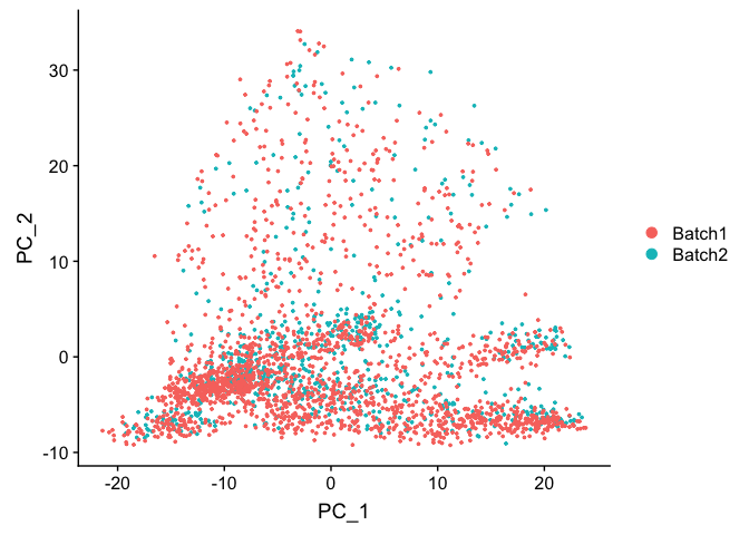
DimPlot(object = experiment.test.noc, group.by = "batchid", reduction = "pca")
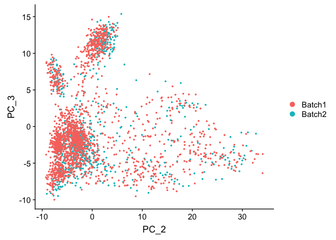
DimPlot(object = experiment.test.noc, group.by = "batchid", dims = c(2,3), reduction = "pca")
PCA Elbow plot to determine how many principal components to use in downstream analyses. Components after the “elbow” in the plot generally explain little additional variability in the data.
ElbowPlot(experiment.test.noc)
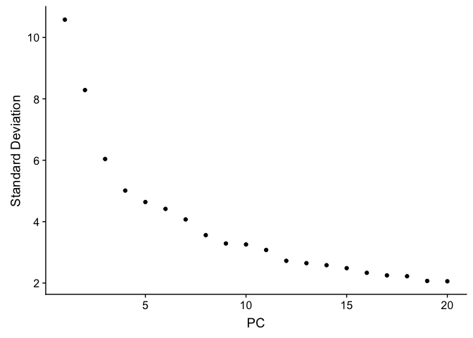
We use 10 components in downstream analyses. Using more components more closely approximates the full data set but increases run time.
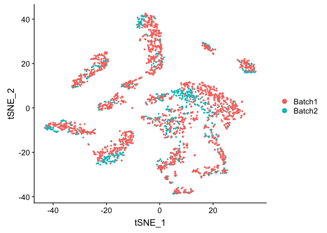
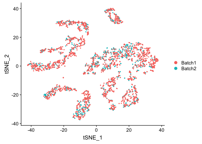
TSNE Plot
pcs.use <- 10
experiment.test.noc <- RunTSNE(object = experiment.test.noc, dims = 1:pcs.use)
DimPlot(object = experiment.test.noc,  group.by = "batchid")
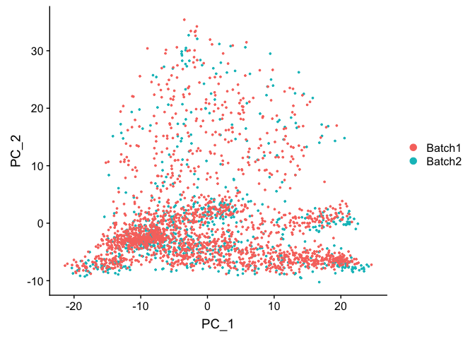
Correct for sample to sample differences (seurat)
Use vars.to.regress to correct for the sample to sample differences and percent mitochondria
experiment.test.regress <- ScaleData(object = experiment.test,
                    vars.to.regress = c("batchid"), model.use = "linear")
Regressing out batchid
Centering and scaling data matrix
experiment.test.regress <- RunPCA(object =experiment.test.regress)
PC_ 1
Positive: Txn1, Sncg, Fez1, S100a10, Atp6v0b, Lxn, Dctn3, Tppp3, Sh3bgrl3, Rabac1
Cisd1, Ppia, Fxyd2, Atp6v1f, Stmn3, Ndufa11, Atp5g1, Bex2, Atpif1, Uchl1
Ndufa4, Psmb6, Ubb, Hagh, Anxa2, Gabarapl2, Rgs10, Nme1, Prdx2, Psmb3
Negative: Mt1, Malat1, Adcyap1, Ptn, Apoe, Zeb2, Mt2, Timp3, Fabp7, Gpm6b
Gal, Kit, Qk, Atp2b4, Plp1, Ifitm3, 6330403K07Rik, Sparc, Id3, Gap43
Gpx3, Selenop, Zfp36l1, Rgcc, Scg2, Cbfb, Zfp36, Igfbp7, Marcksl1, Phlda1
PC_ 2
Positive: Nefh, Cntn1, Thy1, S100b, Sv2b, Cplx1, Slc17a7, Vamp1, Nefm, Lynx1
Endod1, Atp1b1, Scn1a, Nat8l, Vsnl1, Ntrk3, Sh3gl2, Fam19a2, Eno2, Scn1b
Spock1, Scn8a, Glrb, Syt2, Scn4b, Lrrn1, Atp2b2, Lgi3, Cpne6, Snap25
Negative: Malat1, Cd24a, Tmem233, Cd9, Dusp26, Mal2, Tmem158, Carhsp1, Fxyd2, Ctxn3
Ubb, Prkca, Arpc1b, Crip2, S100a6, Gna14, Cd44, Tmem45b, Klf5, Tceal9
Bex3, Hs6st2, Cd82, Emp3, Pfn1, Ift122, Tubb2b, Fam89a, Dynll1, Gadd45g
PC_ 3
Positive: P2ry1, Fam19a4, Gm7271, Rarres1, Th, Zfp521, Wfdc2, Tox3, Gfra2, D130079A08Rik
Iqsec2, Pou4f2, Rgs5, Kcnd3, Id4, Rasgrp1, Slc17a8, Casz1, Cdkn1a, Piezo2
Dpp10, Gm11549, Fxyd6, Rgs10, Spink2, Zfhx3, C1ql4, Cd34, Gabra1, Cckar
Negative: Calca, Basp1, Gap43, Ppp3ca, Map1b, Scg2, Cystm1, Tmem233, Map7d2, Calm1
Ift122, Tubb3, Ncdn, Resp18, Prkca, Etv1, Nmb, Skp1a, Crip2, Epb41l3
Camk2a, Ntrk1, Tspan8, Deptor, Gna14, Adk, Jak1, Tmem255a, Etl4, Camk2g
PC_ 4
Positive: Id3, Timp3, Selenop, Pvalb, Ifitm3, Sparc, Igfbp7, Adk, Tm4sf1, Ly6c1
Sgk1, Id1, Etv1, Nsg1, Mt2, Cldn5, Zfp36l1, Ier2, Itm2a, Spp1
Slc17a7, Aldoc, Ptn, Cxcl12, Shox2, Qk, Stxbp6, Sparcl1, Slit2, Jak1
Negative: Gap43, Calca, Stmn1, Tac1, Ppp3ca, Arhgdig, 6330403K07Rik, Alcam, Prune2, Adcyap1
Kit, Ngfr, Ywhag, Atp1a1, Fxyd6, Gal, Smpd3, Ntrk1, Tmem100, Cd24a
Atp2b4, Mt3, Cnih2, Tppp3, Scn7a, Gpx3, S100a11, Snap25, Gnb1, Cbfb
PC_ 5
Positive: Cpne3, Klf5, Jak1, Acpp, Fxyd2, Nppb, Osmr, Gm525, Htr1f, Sst
Etv1, Nbl1, Rgs4, Zfhx3, Cysltr2, Adk, Tspan8, Npy2r, Nts, Parm1
Tmem233, Prkca, Cd24a, Socs2, Prune2, Il31ra, Dgkz, Ptafr, Gnb1, Ptprk
Negative: Mt1, Ptn, B2m, Dbi, Prdx1, Mt3, Fxyd7, Ifitm3, S100a16, Calca
Id3, Mt2, Pcp4l1, Sparc, Selenop, Ifitm2, Rgcc, Igfbp7, Abcg2, Tm4sf1
Apoe, Selenom, S100a13, Cryab, Hspb1, Timp3, Gap43, Ubb, Ly6c1, Phlda1
DimPlot(object = experiment.test.regress, group.by = "batchid", reduction.use = "pca")
The following functions and any applicable methods accept the dots: CombinePlots
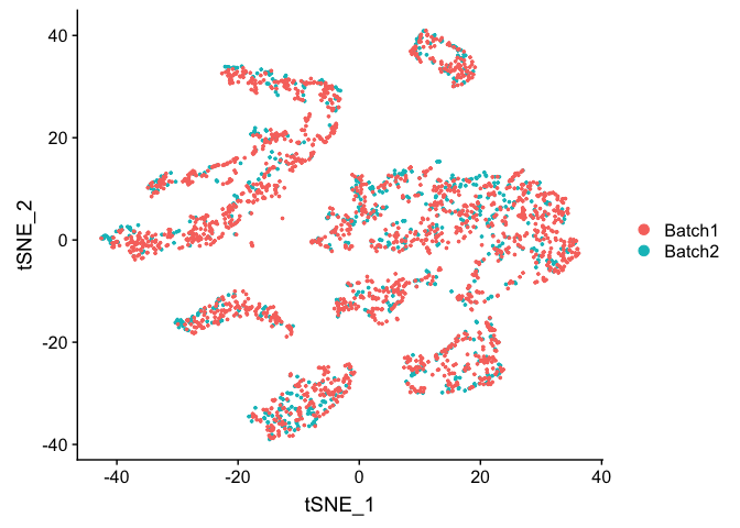
Corrected TSNE Plot
experiment.test.regress <- RunTSNE(object = experiment.test.regress, dims.use = 1:pcs.use)
DimPlot(object = experiment.test.regress, group.by = "batchid", reduction = "tsne")
COMBAT corrected, https://academic.oup.com/biostatistics/article-lookup/doi/10.1093/biostatistics/kxj037
library(sva)
Loading required package: mgcv
Loading required package: nlme
This is mgcv 1.8-31. For overview type 'help("mgcv-package")'.
Loading required package: genefilter
Loading required package: BiocParallel
?ComBat
m = as.matrix(GetAssayData(experiment.test))
com = ComBat(dat=m, batch=as.numeric(as.factor(experiment.test$batchid)), prior.plots=FALSE, par.prior=TRUE)
Found2batches
Adjusting for0covariate(s) or covariate level(s)
Standardizing Data across genes
Fitting L/S model and finding priors
Finding parametric adjustments
Adjusting the Data
experiment.test.combat <- experiment.test
experiment.test.combat <- SetAssayData(experiment.test.combat, new.data = as.matrix(com))
experiment.test.combat = ScaleData(experiment.test.combat)
Centering and scaling data matrix
Principal components on ComBat adjusted data
experiment.test.combat <- RunPCA(object = experiment.test.combat)
PC_ 1
Positive: Txn1, Sncg, Fez1, S100a10, Atp6v0b, Lxn, Dctn3, Tppp3, Sh3bgrl3, Rabac1
Cisd1, Ppia, Fxyd2, Stmn3, Atp6v1f, Ndufa11, Atp5g1, Bex2, Atpif1, Uchl1
Ndufa4, Psmb6, Ubb, Anxa2, Hagh, Gabarapl2, Nme1, Rgs10, Psmb3, Prdx2
Negative: Mt1, Malat1, Adcyap1, Ptn, Apoe, Zeb2, Mt2, Timp3, Fabp7, Gpm6b
Gal, Kit, Qk, Atp2b4, Plp1, Ifitm3, 6330403K07Rik, Sparc, Id3, Gap43
Gpx3, Selenop, Zfp36l1, Rgcc, Scg2, Cbfb, Zfp36, Igfbp7, Marcksl1, Phlda1
PC_ 2
Positive: Nefh, Cntn1, Thy1, S100b, Sv2b, Slc17a7, Cplx1, Vamp1, Nefm, Lynx1
Endod1, Atp1b1, Scn1a, Nat8l, Vsnl1, Ntrk3, Scn8a, Sh3gl2, Fam19a2, Eno2
Scn1b, Spock1, Glrb, Syt2, Scn4b, Lrrn1, Lgi3, Cpne6, Atp2b2, Clec2l
Negative: Malat1, Cd24a, Tmem233, Cd9, Dusp26, Mal2, Tmem158, Carhsp1, Fxyd2, Ubb
Ctxn3, Arpc1b, Crip2, Prkca, S100a6, Gna14, Cd44, Tmem45b, Klf5, Tceal9
Bex3, Hs6st2, Cd82, Emp3, Pfn1, Ift122, Tubb2b, Dynll1, Fam89a, Acpp
PC_ 3
Positive: P2ry1, Fam19a4, Gm7271, Rarres1, Th, Zfp521, Wfdc2, Tox3, Gfra2, D130079A08Rik
Iqsec2, Pou4f2, Rgs5, Kcnd3, Id4, Rasgrp1, Slc17a8, Casz1, Cdkn1a, Piezo2
Dpp10, Gm11549, Fxyd6, Rgs10, Spink2, Zfhx3, C1ql4, Gabra1, Cd34, Cckar
Negative: Calca, Basp1, Gap43, Ppp3ca, Map1b, Scg2, Cystm1, Tmem233, Map7d2, Calm1
Ift122, Ncdn, Tubb3, Prkca, Resp18, Etv1, Skp1a, Nmb, Crip2, Camk2a
Tspan8, Epb41l3, Ntrk1, Gna14, Deptor, Adk, Jak1, Tmem255a, Etl4, Camk2g
PC_ 4
Positive: Id3, Timp3, Pvalb, Selenop, Sparc, Ifitm3, Igfbp7, Adk, Tm4sf1, Etv1
Sgk1, Ly6c1, Id1, Nsg1, Mt2, Slc17a7, Spp1, Zfp36l1, Cldn5, Ier2
Aldoc, Shox2, Itm2a, Ptn, Stxbp6, Cxcl12, Qk, Jak1, Slit2, Sparcl1
Negative: Gap43, Calca, Stmn1, Tac1, Ppp3ca, Arhgdig, 6330403K07Rik, Alcam, Adcyap1, Prune2
Ngfr, Kit, Ywhag, Atp1a1, Gal, Fxyd6, Smpd3, Ntrk1, Tmem100, Mt3
Cd24a, Atp2b4, Cnih2, Tppp3, S100a11, Gpx3, Scn7a, Cbfb, Snap25, Gnb1
PC_ 5
Positive: Cpne3, Klf5, Acpp, Fxyd2, Jak1, Nppb, Osmr, Gm525, Htr1f, Sst
Nbl1, Etv1, Rgs4, Zfhx3, Cysltr2, Tspan8, Adk, Npy2r, Parm1, Tmem233
Nts, Cd24a, Prkca, Prune2, Socs2, Il31ra, Dgkz, Gnb1, Phf24, Ptafr
Negative: Mt1, Ptn, B2m, Prdx1, Dbi, Mt3, Ifitm3, Fxyd7, S100a16, Id3
Calca, Mt2, Sparc, Pcp4l1, Selenop, Ifitm2, Rgcc, Igfbp7, Apoe, Tm4sf1
Abcg2, Cryab, Selenom, S100a13, Ubb, Timp3, Hspb1, Phlda1, Ly6c1, Dad1
DimPlot(object = experiment.test.combat, group.by = "batchid", reduction = "pca")
TSNE plot on ComBat adjusted data
experiment.test.combat <- RunTSNE(object = experiment.test.combat, dims.use = 1:pcs.use)
DimPlot(object = experiment.test.combat, group.by = "batchid", reduction = "tsne")
Question(s)
- Try a couple of PCA cutoffs (low and high) and compare the TSNE plots from the different methods. Do they look meaningfully different?
Get the next Rmd file
download.file("https://raw.githubusercontent.com/ucdavis-bioinformatics-training/2019-single-cell-RNA-sequencing-Workshop-UCD_UCSF/master/scrnaseq_analysis/scRNA_Workshop-PART4.Rmd", "scRNA_Workshop-PART4.Rmd")
Session Information
sessionInfo()
R version 3.5.1 (2018-07-02)
Platform: x86_64-apple-darwin16.7.0 (64-bit)
Running under: macOS 10.14.5
Matrix products: default
BLAS: /System/Library/Frameworks/Accelerate.framework/Versions/A/Frameworks/vecLib.framework/Versions/A/libBLAS.dylib
LAPACK: /System/Library/Frameworks/Accelerate.framework/Versions/A/Frameworks/vecLib.framework/Versions/A/libLAPACK.dylib
locale:
[1] en_US.UTF-8/en_US.UTF-8/en_US.UTF-8/C/en_US.UTF-8/en_US.UTF-8
attached base packages:
[1] stats graphics grDevices utils datasets methods base
other attached packages:
[1] sva_3.30.1 BiocParallel_1.16.6 genefilter_1.64.0
[4] mgcv_1.8-31 nlme_3.1-142 Seurat_3.1.1
loaded via a namespace (and not attached):
[1] Rtsne_0.15 colorspace_1.4-1 ggridges_0.5.1
[4] leiden_0.3.1 listenv_0.7.0 farver_2.0.1
[7] npsurv_0.4-0 ggrepel_0.8.1 bit64_0.9-7
[10] AnnotationDbi_1.44.0 codetools_0.2-16 splines_3.5.1
[13] R.methodsS3_1.7.1 lsei_1.2-0 knitr_1.26
[16] zeallot_0.1.0 jsonlite_1.6 annotate_1.60.1
[19] ica_1.0-2 cluster_2.1.0 png_0.1-7
[22] R.oo_1.23.0 uwot_0.1.4 sctransform_0.2.0
[25] compiler_3.5.1 httr_1.4.1 backports_1.1.5
[28] assertthat_0.2.1 Matrix_1.2-17 lazyeval_0.2.2
[31] limma_3.38.3 htmltools_0.4.0 tools_3.5.1
[34] rsvd_1.0.2 igraph_1.2.4.1 gtable_0.3.0
[37] glue_1.3.1 RANN_2.6.1 reshape2_1.4.3
[40] dplyr_0.8.3 Rcpp_1.0.3 Biobase_2.42.0
[43] vctrs_0.2.0 gdata_2.18.0 ape_5.3
[46] gbRd_0.4-11 lmtest_0.9-37 xfun_0.11
[49] stringr_1.4.0 globals_0.12.4 lifecycle_0.1.0
[52] irlba_2.3.3 gtools_3.8.1 XML_3.98-1.20
[55] future_1.15.1 MASS_7.3-51.4 zoo_1.8-6
[58] scales_1.1.0 parallel_3.5.1 RColorBrewer_1.1-2
[61] yaml_2.2.0 memoise_1.1.0 reticulate_1.13
[64] pbapply_1.4-2 gridExtra_2.3 ggplot2_3.2.1
[67] stringi_1.4.3 RSQLite_2.1.2 highr_0.8
[70] S4Vectors_0.20.1 caTools_1.17.1.2 BiocGenerics_0.28.0
[73] bibtex_0.4.2 matrixStats_0.55.0 Rdpack_0.11-0
[76] SDMTools_1.1-221.1 rlang_0.4.2.9000 pkgconfig_2.0.3
[79] bitops_1.0-6 evaluate_0.14 lattice_0.20-38
[82] ROCR_1.0-7 purrr_0.3.3 htmlwidgets_1.5.1
[85] labeling_0.3 bit_1.1-14 cowplot_1.0.0
[88] tidyselect_0.2.5 RcppAnnoy_0.0.14 plyr_1.8.4
[91] magrittr_1.5 R6_2.4.1 IRanges_2.16.0
[94] gplots_3.0.1.1 DBI_1.0.0 pillar_1.4.2
[97] fitdistrplus_1.0-14 survival_3.1-7 RCurl_1.95-4.12
[100] tibble_2.1.3 future.apply_1.3.0 tsne_0.1-3
[103] crayon_1.3.4 KernSmooth_2.23-16 plotly_4.9.1
[106] rmarkdown_1.17 grid_3.5.1 data.table_1.12.6
[109] blob_1.2.0 metap_1.1 digest_0.6.23
[112] xtable_1.8-4 tidyr_1.0.0 R.utils_2.9.0
[115] RcppParallel_4.4.4 stats4_3.5.1 munsell_0.5.0
[118] viridisLite_0.3.0