Reminder of samples
- UCD_Adj_VitE
- UCD_Supp_VitE
- UCD_VitE_Def
Load libraries
library(Seurat)
library(ggplot2)
Load the Seurat object
load("clusters_seurat_object.RData")
experiment.merged
An object of class Seurat
12811 features across 2681 samples within 1 assay
Active assay: RNA (12811 features)
2 dimensional reductions calculated: pca, tsne
Idents(experiment.merged) <- "RNA_snn_res.0.5"
#0. Setup
Load the final Seurat object, load libraries (also see additional required packages for each example)
#1. DE With Single Cell Data Using Limma
For differential expression using models more complex than those allowed by FindAllMarkers(), data from Seurat may be used in limma (https://www.bioconductor.org/packages/devel/bioc/vignettes/limma/inst/doc/usersguide.pdf)
We illustrate by comparing sample 1 to sample 2 within cluster 0:
library(limma)
cluster0 <- subset(experiment.merged, idents = '0')
expr <- as.matrix(GetAssayData(cluster0))

# Filter out genes that are 0 for every cell in this cluster
bad <- which(rowSums(expr) == 0)
expr <- expr[-bad,]

mm <- model.matrix(~0 + orig.ident, data = cluster0@meta.data)
fit <- lmFit(expr, mm)
head(coef(fit)) # means in each sample for each gene
orig.identUCD_Adj_VitE orig.identUCD_Supp_VitE orig.identUCD_VitE_Def
Xkr4 0.00000000 0.00000000 0.01205985
Sox17 0.00000000 0.01640103 0.00000000
Mrpl15 0.08176912 0.03491121 0.09928512
Lypla1 0.19102070 0.14113531 0.27421545
Tcea1 0.20114933 0.20678820 0.19408342
Rgs20 0.08977786 0.16413658 0.12434977
contr <- makeContrasts(orig.identUCD_Supp_VitE - orig.identUCD_Adj_VitE, levels = colnames(coef(fit)))
tmp <- contrasts.fit(fit, contrasts = contr)
tmp <- eBayes(tmp)
topTable(tmp, sort.by = "P", n = 20) # top 20 DE genes
logFC AveExpr t P.Value adj.P.Val B
Rpl21 -0.7724848 2.14209018 -5.890378 7.159580e-09 0.0000851632 9.738313
Rpl23a -0.6865649 2.16173396 -5.447342 8.100825e-08 0.0004817966 7.531265
Pcp4 -0.8229684 1.93476081 -5.256214 2.197765e-07 0.0006546034 6.625881
Rpl17 -0.6834796 2.01758975 -5.255904 2.201273e-07 0.0006546034 6.624435
Tmsb10 -0.5450433 3.35838422 -5.050790 6.215190e-07 0.0014785938 5.684808
Rpl24 -0.5851214 2.09652619 -4.725294 3.005267e-06 0.0053603951 4.262728
H3f3b -0.6036830 2.25676617 -4.714988 3.154499e-06 0.0053603951 4.219097
Rpl39 -0.5342677 2.23529589 -4.415747 1.239149e-05 0.0184246007 2.990268
Rps8 -0.5492130 2.51810086 -4.333518 1.780959e-05 0.0189443296 2.665539
Ndufa3 -0.4830157 0.75072369 -4.325111 1.847651e-05 0.0189443296 2.632655
Rpl32 -0.5540049 2.44843495 -4.323717 1.858932e-05 0.0189443296 2.627210
Zfp467 -0.2498323 0.16203051 -4.317371 1.911156e-05 0.0189443296 2.602431
Tshz2 -0.5507727 2.31127549 -4.247578 2.586002e-05 0.0236619148 2.332172
Rps15 -0.5515529 1.97711264 -4.207744 3.067469e-05 0.0250844004 2.179746
Tmsb4x -0.3744138 3.22966552 -4.200539 3.163228e-05 0.0250844004 2.152316
Alkal2 -0.1394787 0.05421123 -4.180105 3.450525e-05 0.0256524996 2.074765
Rpl10 -0.4858114 2.22403787 -4.042487 6.139313e-05 0.0429571322 1.561626
Rps24 -0.5126108 1.51587449 -4.002111 7.247695e-05 0.0465589355 1.414108
Rpl9 -0.4899921 2.44944433 -3.982811 7.842255e-05 0.0465589355 1.344080
Dbpht2 -0.4185910 0.61581149 -3.975239 8.087904e-05 0.0465589355 1.316694
- logFC: log2 fold change (UCD_Supp_VitE/UCD_Adj_VitE)
- AveExpr: Average expression, in log2 counts per million, across all cells included in analysis (i.e. those in cluster 0)
- t: t-statistic, i.e. logFC divided by its standard error
- P.Value: Raw p-value from test that logFC differs from 0
- adj.P.Val: Benjamini-Hochberg false discovery rate adjusted p-value
The limma vignette linked above gives more detail on model specification.
2. Gene Ontology (GO) Enrichment of Genes Expressed in a Cluster
Loading required package: BiocGenerics
Loading required package: parallel
Attaching package: 'BiocGenerics'
The following objects are masked from 'package:parallel':
clusterApply, clusterApplyLB, clusterCall, clusterEvalQ, clusterExport, clusterMap, parApply, parCapply, parLapply, parLapplyLB, parRapply, parSapply, parSapplyLB
The following object is masked from 'package:limma':
plotMA
The following objects are masked from 'package:stats':
IQR, mad, sd, var, xtabs
The following objects are masked from 'package:base':
anyDuplicated, append, as.data.frame, basename, cbind, colnames, dirname, do.call, duplicated, eval, evalq, Filter, Find, get, grep, grepl, intersect, is.unsorted, lapply, Map, mapply, match, mget, order, paste, pmax, pmax.int, pmin, pmin.int, Position, rank, rbind, Reduce, rownames, sapply, setdiff, sort, table, tapply, union, unique, unsplit, which, which.max, which.min
Loading required package: graph
Loading required package: Biobase
Welcome to Bioconductor
Vignettes contain introductory material; view with 'browseVignettes()'. To cite Bioconductor, see 'citation("Biobase")', and for packages 'citation("pkgname")'.
Loading required package: GO.db
Loading required package: AnnotationDbi
Loading required package: stats4
Loading required package: IRanges
Loading required package: S4Vectors
Attaching package: 'S4Vectors'
The following object is masked from 'package:base':
expand.grid
Loading required package: SparseM
Attaching package: 'SparseM'
The following object is masked from 'package:base':
backsolve
groupGOTerms: GOBPTerm, GOMFTerm, GOCCTerm environments built.
Attaching package: 'topGO'
The following object is masked from 'package:IRanges':
members
# install org.Mm.eg.db from Bioconductor if not already installed (for mouse only)
cluster0 <- subset(experiment.merged, idents = '0')
expr <- as.matrix(GetAssayData(cluster0))
# Select genes that are expressed > 0 in at least 75% of cells (somewhat arbitrary definition)
n.gt.0 <- apply(expr, 1, function(x)length(which(x > 0)))
expressed.genes <- rownames(expr)[which(n.gt.0/ncol(expr) >= 0.75)]
all.genes <- rownames(expr)

# define geneList as 1 if gene is in expressed.genes, 0 otherwise
geneList <- ifelse(all.genes %in% expressed.genes, 1, 0)
names(geneList) <- all.genes

# Create topGOdata object
	GOdata <- new("topGOdata",
		ontology = "BP", # use biological process ontology
		allGenes = geneList,
		geneSelectionFun = function(x)(x == 1),
              annot = annFUN.org, mapping = "org.Mm.eg.db", ID = "symbol")
Building most specific GOs .....
Loading required package: org.Mm.eg.db
( 10570 GO terms found. )
Build GO DAG topology ..........
( 14604 GO terms and 34657 relations. )
Annotating nodes ...............
( 11727 genes annotated to the GO terms. )
# Test for enrichment using Fisher's Exact Test
	resultFisher <- runTest(GOdata, algorithm = "elim", statistic = "fisher")
-- Elim Algorithm --
the algorithm is scoring 2878 nontrivial nodes
parameters:
test statistic: fisher
cutOff: 0.01
Level 19: 1 nodes to be scored (0 eliminated genes)
Level 18: 1 nodes to be scored (0 eliminated genes)
Level 17: 1 nodes to be scored (0 eliminated genes)
Level 16: 6 nodes to be scored (0 eliminated genes)
Level 15: 15 nodes to be scored (0 eliminated genes)
Level 14: 32 nodes to be scored (13 eliminated genes)
Level 13: 73 nodes to be scored (20 eliminated genes)
Level 12: 110 nodes to be scored (416 eliminated genes)
Level 11: 180 nodes to be scored (750 eliminated genes)
Level 10: 256 nodes to be scored (778 eliminated genes)
Level 9: 325 nodes to be scored (1419 eliminated genes)
Level 8: 379 nodes to be scored (1555 eliminated genes)
Level 7: 453 nodes to be scored (2045 eliminated genes)
Level 6: 441 nodes to be scored (2267 eliminated genes)
Level 5: 323 nodes to be scored (2327 eliminated genes)
Level 4: 180 nodes to be scored (2328 eliminated genes)
Level 3: 83 nodes to be scored (2974 eliminated genes)
Level 2: 18 nodes to be scored (3547 eliminated genes)
Level 1: 1 nodes to be scored (3547 eliminated genes)
GenTable(GOdata, Fisher = resultFisher, topNodes = 20, numChar = 60)
GO.ID Term Annotated Significant Expected Fisher
1 GO:0006412 translation 517 48 5.73 9.1e-19
2 GO:0002181 cytoplasmic translation 77 17 0.85 5.5e-18
3 GO:0000028 ribosomal small subunit assembly 18 7 0.20 5.0e-10
4 GO:0000027 ribosomal large subunit assembly 29 7 0.32 2.2e-08
5 GO:0097214 positive regulation of lysosomal membrane permeability 2 2 0.02 0.00012
6 GO:0000462 maturation of SSU-rRNA from tricistronic rRNA transcript (SS... 30 4 0.33 0.00032
7 GO:0006880 intracellular sequestering of iron ion 3 2 0.03 0.00036
8 GO:0016198 axon choice point recognition 4 2 0.04 0.00072
9 GO:0061844 antimicrobial humoral immune response mediated by antimicrob... 17 3 0.19 0.00081
10 GO:0006605 protein targeting 230 9 2.55 0.00104
11 GO:0071635 negative regulation of transforming growth factor beta produ... 5 2 0.06 0.00119
12 GO:0002227 innate immune response in mucosa 5 2 0.06 0.00119
13 GO:0007409 axonogenesis 353 13 3.91 0.00151
14 GO:0002679 respiratory burst involved in defense response 6 2 0.07 0.00178
15 GO:1902255 positive regulation of intrinsic apoptotic signaling pathway... 6 2 0.07 0.00178
16 GO:1905323 telomerase holoenzyme complex assembly 6 2 0.07 0.00178
17 GO:1904667 negative regulation of ubiquitin protein ligase activity 7 2 0.08 0.00247
18 GO:0071637 regulation of monocyte chemotactic protein-1 production 7 2 0.08 0.00247
19 GO:0048588 developmental cell growth 213 8 2.36 0.00254
20 GO:0050808 synapse organization 371 11 4.11 0.00276
- Annotated: number of genes (out of all.genes) that are annotated with that GO term
- Significant: number of genes that are annotated with that GO term and meet our criteria for “expressed”
- Expected: Under random chance, number of genes that would be expected to be annotated with that GO term and meeting our criteria for “expressed”
- Fisher: (Raw) p-value from Fisher’s Exact Test
#3. Weighted Gene Co-Expression Network Analysis (WGCNA)
WGCNA identifies groups of genes (“modules”) with correlated expression.
WARNING: TAKES A LONG TIME TO RUN
Loading required package: dynamicTreeCut
Loading required package: fastcluster
Attaching package: 'fastcluster'
The following object is masked from 'package:stats':
hclust
Attaching package: 'WGCNA'
The following object is masked from 'package:IRanges':
cor
The following object is masked from 'package:S4Vectors':
cor
The following object is masked from 'package:stats':
cor
options(stringsAsFactors = F)
datExpr <- t(as.matrix(GetAssayData(experiment.merged)))[,VariableFeatures(experiment.merged)]  # only use variable genes in analysis

net <- blockwiseModules(datExpr, power = 10,
  corType = "bicor", # use robust correlation
	networkType = "signed", minModuleSize = 10,
	reassignThreshold = 0, mergeCutHeight = 0.15,
	numericLabels = F, pamRespectsDendro = FALSE,
	saveTOMs = TRUE,
	saveTOMFileBase = "TOM",
	verbose = 3)
Calculating module eigengenes block-wise from all genes
Flagging genes and samples with too many missing values...
..step 1
..Working on block 1 .
TOM calculation: adjacency..
..will not use multithreading.
alpha: 1.000000
Fraction of slow calculations: 0.000000
..connectivity..
..matrix multiplication (system BLAS)..
..normalization..
..done.
..saving TOM for block 1 into file TOM-block.1.RData
....clustering..
....detecting modules..
....calculating module eigengenes..
....checking kME in modules..
..removing 67 genes from module 1 because their KME is too low.
..removing 43 genes from module 3 because their KME is too low.
..removing 2 genes from module 12 because their KME is too low.
..merging modules that are too close..
mergeCloseModules: Merging modules whose distance is less than 0.15
alpha: 1.000000
Calculating new MEs...
alpha: 1.000000
black blue brown green grey red turquoise yellow
11 80 21 12 1536 11 312 17
# Convert labels to colors for plotting
mergedColors = net$colors
# Plot the dendrogram and the module colors underneath
plotDendroAndColors(net$dendrograms[[1]], mergedColors[net$blockGenes[[1]]],
"Module colors",
dendroLabels = FALSE, hang = 0.03,
addGuide = TRUE, guideHang = 0.05)
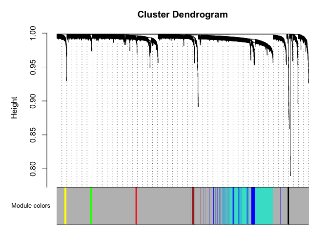 Genes in grey module are unclustered.
What genes are in the “blue” module?
colnames(datExpr)[net$colors == "blue"]
[1] "Lxn" "Txn1" "Grik1" "Fez1" "Tmem45b" "Synpr" "Tceal9" "Ppp1r1a" "Rgs10" "Nrn1" "Fxyd2" "Ostf1" "Lix1" "Sncb" "Paqr5" "Bex3" "Anxa5" "Gfra2" "Scg3" "Ppm1j" "Kcnab1" "Kcnip4" "Cadm1" "Isl2" "Pla2g7" "Tppp3" "Rgs4"
[28] "Tmsb4x" "Unc119" "Pmm1" "Ccdc68" "Rnf7" "Prr13" "Rsu1" "Pmp22" "Acpp" "Kcnip2" "Cdk15" "Mrps6" "Ebp" "Hexb" "Cdh11" "Dapk2" "Ano3" "Pde6d" "Snx7" "Dtnbp1" "Tubb2b" "Nr2c2ap" "Phf24" "Rcan2" "Fam241b" "Pmvk" "Slc25a4"
[55] "Zfhx3" "Dgkz" "Ndufv1" "Ptrh1" "1700037H04Rik" "Kif5b" "Sae1" "Sri" "Cpne3" "Dgcr6" "Cisd3" "Syt7" "Lhfpl3" "Dda1" "Ppp1ca" "Glrx3" "Stoml1" "Plagl1" "Lbh" "Degs1" "AI413582" "Car10" "Tlx2" "Parm1" "March11" "Cpe"
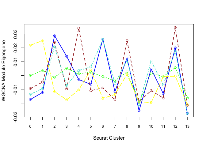
Each cluster is represented by a summary “eigengene”.
Plot eigengenes for each non-grey module by clusters from Seurat:
f <- function(module){
  eigengene <- unlist(net$MEs[paste0("ME", module)])
  means <- tapply(eigengene, Idents(experiment.merged), mean, na.rm = T)
  return(means)
}
modules <- c("blue", "brown", "green", "turquoise", "yellow")
plotdat <- sapply(modules, f)
matplot(plotdat, col = modules, type = "l", lwd = 2, xaxt = "n", xlab = "Seurat Cluster",
        ylab = "WGCNA Module Eigengene")
axis(1, at = 1:19, labels = 0:18, cex.axis = 0.8)
matpoints(plotdat, col = modules, pch = 21)
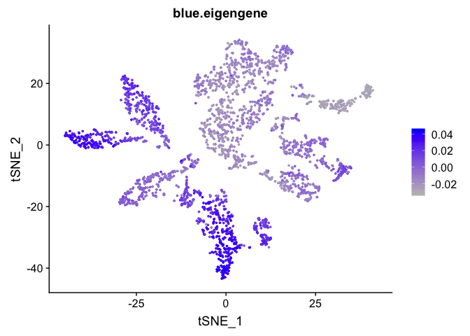
Can also plot the module onto the tsne plot
blue.eigengene <- unlist(net$MEs[paste0("ME", "blue")])
names(blue.eigengene) <- rownames(datExpr)
experiment.merged$blue.eigengene <- blue.eigengene
FeaturePlot(experiment.merged, features = "blue.eigengene", cols = c("grey", "blue"))
Get the next Rmd file
download.file("https://raw.githubusercontent.com/ucdavis-bioinformatics-training/2019-single-cell-RNA-sequencing-Workshop-UCD_UCSF/master/scrnaseq_analysis/scRNA_Workshop-PART7.Rmd", "scRNA_Workshop-PART7.Rmd")
R version 3.6.0 (2019-04-26)
Platform: x86_64-apple-darwin15.6.0 (64-bit)
Running under: macOS Mojave 10.14.5
Matrix products: default
BLAS: /Library/Frameworks/R.framework/Versions/3.6/Resources/lib/libRblas.0.dylib
LAPACK: /Library/Frameworks/R.framework/Versions/3.6/Resources/lib/libRlapack.dylib
locale:
[1] en_US.UTF-8/en_US.UTF-8/en_US.UTF-8/C/en_US.UTF-8/en_US.UTF-8
attached base packages:
[1] stats4 parallel stats graphics grDevices utils datasets methods base
other attached packages:
[1] WGCNA_1.68 fastcluster_1.1.25 dynamicTreeCut_1.63-1 org.Mm.eg.db_3.8.2 topGO_2.36.0 SparseM_1.77 GO.db_3.8.2 AnnotationDbi_1.46.0 IRanges_2.18.1 S4Vectors_0.22.0 Biobase_2.44.0 graph_1.62.0 BiocGenerics_0.30.0 limma_3.40.2 ggplot2_3.2.0 Seurat_3.0.2
loaded via a namespace (and not attached):
[1] backports_1.1.4 Hmisc_4.2-0 plyr_1.8.4 igraph_1.2.4.1 lazyeval_0.2.2 splines_3.6.0 listenv_0.7.0 robust_0.4-18 digest_0.6.19 foreach_1.4.4 htmltools_0.3.6 gdata_2.18.0 magrittr_1.5 checkmate_1.9.3 memoise_1.1.0 fit.models_0.5-14 cluster_2.1.0 doParallel_1.0.14 ROCR_1.0-7 globals_0.12.4
[21] matrixStats_0.54.0 R.utils_2.9.0 colorspace_1.4-1 blob_1.1.1 rrcov_1.4-7 ggrepel_0.8.1 xfun_0.7 dplyr_0.8.1 crayon_1.3.4 jsonlite_1.6 impute_1.58.0 survival_2.44-1.1 zoo_1.8-6 iterators_1.0.10 ape_5.3 glue_1.3.1 gtable_0.3.0 future.apply_1.3.0 DEoptimR_1.0-8 scales_1.0.0
[41] mvtnorm_1.0-11 DBI_1.0.0 bibtex_0.4.2 Rcpp_1.0.1 metap_1.1 viridisLite_0.3.0 htmlTable_1.13.1 reticulate_1.12 foreign_0.8-71 bit_1.1-14 rsvd_1.0.1 SDMTools_1.1-221.1 preprocessCore_1.46.0 Formula_1.2-3 tsne_0.1-3 htmlwidgets_1.3 httr_1.4.0 gplots_3.0.1.1 RColorBrewer_1.1-2 acepack_1.4.1
[61] ica_1.0-2 pkgconfig_2.0.2 R.methodsS3_1.7.1 nnet_7.3-12 tidyselect_0.2.5 labeling_0.3 rlang_0.3.4 reshape2_1.4.3 munsell_0.5.0 tools_3.6.0 RSQLite_2.1.1 ggridges_0.5.1 evaluate_0.14 stringr_1.4.0 yaml_2.2.0 npsurv_0.4-0 knitr_1.23 bit64_0.9-7 fitdistrplus_1.0-14 robustbase_0.93-5
[81] caTools_1.17.1.2 purrr_0.3.2 RANN_2.6.1 pbapply_1.4-0 future_1.13.0 nlme_3.1-140 R.oo_1.22.0 compiler_3.6.0 rstudioapi_0.10 plotly_4.9.0 png_0.1-7 lsei_1.2-0 tibble_2.1.3 pcaPP_1.9-73 stringi_1.4.3 lattice_0.20-38 Matrix_1.2-17 pillar_1.4.1 Rdpack_0.11-0 lmtest_0.9-37
[101] data.table_1.12.2 cowplot_0.9.4 bitops_1.0-6 irlba_2.3.3 gbRd_0.4-11 R6_2.4.0 latticeExtra_0.6-28 KernSmooth_2.23-15 gridExtra_2.3 codetools_0.2-16 MASS_7.3-51.4 gtools_3.8.1 assertthat_0.2.1 withr_2.1.2 sctransform_0.2.0 grid_3.6.0 rpart_4.1-15 tidyr_0.8.3 rmarkdown_1.13 Rtsne_0.15
[121] base64enc_0.1-3
