</div>
### Are there any T/B cells out there??
```r
table(!is.na(s_balbc_pbmc$t_clonotype_id),!is.na(s_balbc_pbmc$b_clonotype_id))
```
FALSE TRUE
FALSE 1074 4488
TRUE 2175 220
```r
s_balbc_pbmc <- subset(s_balbc_pbmc, cells = colnames(s_balbc_pbmc)[!(!is.na(s_balbc_pbmc$t_clonotype_id) &
!is.na(s_balbc_pbmc$b_clonotype_id))])
s_balbc_pbmc
```
An object of class Seurat
15975 features across 7737 samples within 1 assay
Active assay: RNA (15975 features, 0 variable features)
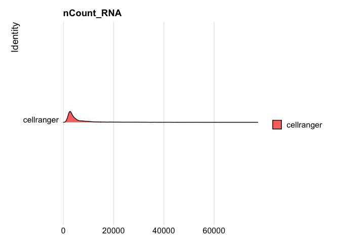
### Lets take a look at some other metadata
```r
RidgePlot(s_balbc_pbmc, features="nCount_RNA")
```
Picking joint bandwidth of 439
```r
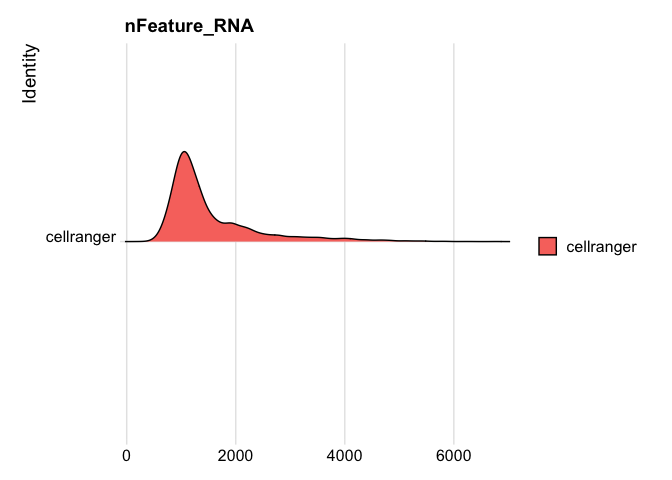
RidgePlot(s_balbc_pbmc, features="nFeature_RNA")
```
Picking joint bandwidth of 86.1
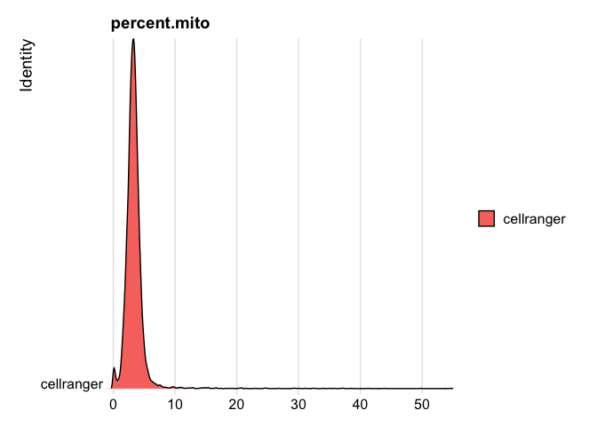
```r
RidgePlot(s_balbc_pbmc, features="percent.mito")
```
Picking joint bandwidth of 0.132
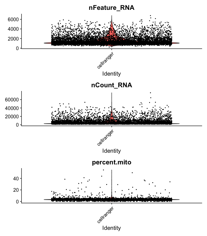
```r
VlnPlot(
s_balbc_pbmc,
features = c("nFeature_RNA", "nCount_RNA","percent.mito"),
ncol = 1, pt.size = 0.3)
```
```r
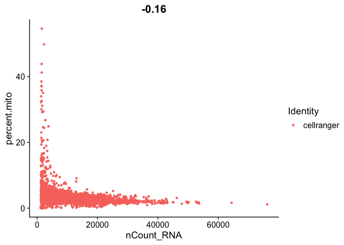
FeatureScatter(s_balbc_pbmc, feature1 = "nCount_RNA", feature2 = "percent.mito")
```
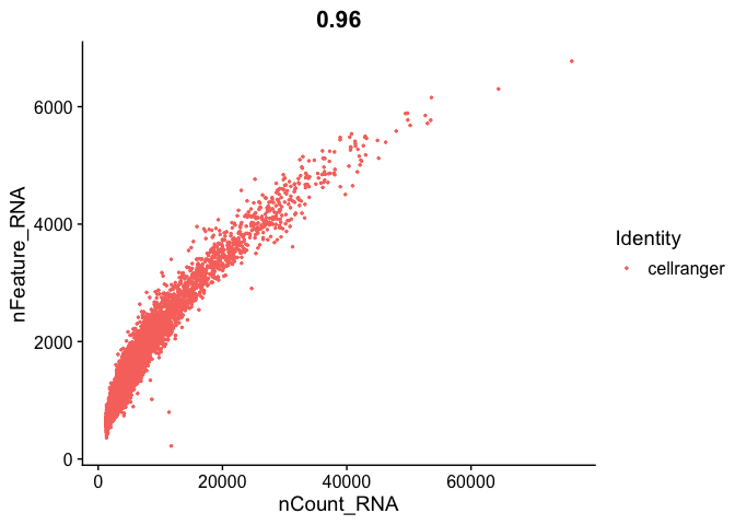
```r
FeatureScatter(s_balbc_pbmc, "nCount_RNA", "nFeature_RNA",pt.size = 0.5)
```
```r
s_balbc_pbmc <- subset(s_balbc_pbmc, percent.mito <= 10)
s_balbc_pbmc <- subset(s_balbc_pbmc, nCount_RNA >= 500 & nCount_RNA <= 40000)
s_balbc_pbmc
```
An object of class Seurat
15975 features across 7634 samples within 1 assay
Active assay: RNA (15975 features, 0 variable features)
```r
s_balbc_pbmc <- NormalizeData(s_balbc_pbmc, normalization.method = "LogNormalize", scale.factor = 10000)
s_balbc_pbmc <- FindVariableFeatures(s_balbc_pbmc, selection.method = "vst", nfeatures = 2000)
all.genes <- rownames(s_balbc_pbmc)
s_balbc_pbmc <- ScaleData(s_balbc_pbmc, features = all.genes)
```
Centering and scaling data matrix
```r
s_balbc_pbmc <- RunPCA(s_balbc_pbmc, features = VariableFeatures(object = s_balbc_pbmc))
```
PC_ 1
Positive: Ighm, Igkc, Mzb1, H2-Eb1, H2-Aa, Cd74, H2-Ab1, Trbc2, Ms4a4b, Cd72
Gm30211, Tcf7, Vpreb3, Il7r, Ly6d, Hmgb2, Thy1, Iglc1, Ass1, Rrad
Dapl1, AW112010, Trbc1, Cd8b1, Sh2d1a, Itm2a, Hs3st1, Fam129c, Ctsw, Gata3
Negative: Fn1, Emilin2, Lyz2, Cxcl2, App, Fcgr3, Ccl6, Sdc3, Wfdc17, Itgam
Ltc4s, Lrp1, Alox5ap, Mt1, Csf1r, Cd14, Cxcl1, Ptgs1, Ifitm3, Ier3
Plxdc2, Ccl9, Ccl24, Cfp, Trf, Fgfr1, Ednrb, S100a1, Ifitm2, Gda
PC_ 2
Positive: Prg4, Cd5l, Alox15, Ptgis, Selp, Ltbp1, Saa3, Garnl3, Pmp22, C1qc
C1qa, C1qb, Ednrb, C4b, Tgfb2, Fcna, Icam2, Itga6, Adgre1, Serpinb2
Gm16104, Bcam, Serpine1, Flnb, Timd4, Padi4, F10, Gm10369, Gata6, Emilin1
Negative: Il1b, Lst1, Gm5150, Sirpb1c, Ltb4r1, Ccr2, Cd300c2, Clec4a2, Csf3r, S100a9
Mmp9, Fam129a, Hp, Il1r2, Cxcr2, S100a8, Cass4, Clec4b1, Plbd1, Clec4a3
Fgr, Jaml, Ptafr, Msrb1, Tmem176b, Cd300lf, Clec4a1, Tnip3, Gcnt2, Bcl2a1a
PC_ 3
Positive: S100a9, S100a8, Csf3r, Cxcr2, Hdc, Hp, Retnlg, Il1r2, Cd33, Gcnt2
Slfn4, Mmp9, Slfn1, Tnfaip2, Trem1, Arg2, Slc40a1, Lst1, Trem3, Cd300lf
F630028O10Rik, Pygl, Ccr1, Lrg1, Selplg, Clec4d, Stfa2l1, Rnf149, Ifitm1, Gm5150
Negative: Cd74, H2-Eb1, H2-Aa, H2-Ab1, Slamf9, Crip1, Rassf4, Capg, Ighm, Pld4
Plac8, Mrc1, Mzb1, Clec4b1, Tubb6, Tnip3, Ctss, Fcrls, Tmem176b, Ahnak
Tmem176a, Igkc, S100a4, Tppp3, Zbtb32, Ctsz, Ccr2, Cysltr1, Hopx, Batf3
PC_ 4
Positive: Cd74, Ighm, H2-Aa, Igkc, H2-Eb1, Mzb1, H2-Ab1, Plac8, Iglc1, Aldh2
Ly6e, Capg, Cst3, Cyp4f18, Gm30211, Ctsz, Ly6d, Spi1, S100a6, Zbtb32
Ctss, Cyba, Rassf4, Plaur, Pld4, Ncf4, Sox5, Atf3, Vpreb3, S100a8
Negative: Ms4a4b, Trbc2, Thy1, Tcf7, Il7r, Dok2, Fxyd5, Ctsw, Nkg7, Rgs10
Il2rb, Npc2, Selplg, AW112010, Klk8, Sh2d1a, Id2, Trbc1, Ccl5, Ramp1
Cd7, Ccr2, Cd8b1, Gata3, Klrd1, Lcp2, Ppp1r15a, Dapl1, Igfbp4, Cd226
PC_ 5
Positive: Pclaf, Birc5, Mki67, Spc24, Cdk1, Cdca3, Ube2c, Nusap1, Ccna2, Cenpm
Tpx2, Ccnb2, Rrm2, Pbk, Tyms, Cdca8, Cenpf, Ckap2l, Kif11, Tk1
Clspn, Uhrf1, Top2a, Esco2, Bub1, Kif15, Cks1b, Shcbp1, Bub1b, Prc1
Negative: Pid1, Krt80, Lyz1, Retnla, Clec4a1, Ifitm6, Ccr2, Gm21188, Gm36161, Plcb1
Abca9, Kazald1, Tmem176b, Tmem176a, Pltp, Il6, Gm41307, Kank3, Clec4a3, Fcrls
Ltb4r1, Clec4b1, Ccl9, Mrc1, Ms4a8a, Ecm1, Mcub, Tifab, Dapk1, Fcgrt
```r
use.pcs = 1:30
s_balbc_pbmc <- FindNeighbors(s_balbc_pbmc, dims = use.pcs)
```
Computing nearest neighbor graph
Computing SNN
```r
s_balbc_pbmc <- FindClusters(s_balbc_pbmc, resolution = c(0.5))
```
Modularity Optimizer version 1.3.0 by Ludo Waltman and Nees Jan van Eck
Number of nodes: 7634
Number of edges: 332010
Running Louvain algorithm...
Maximum modularity in 10 random starts: 0.9037
Number of communities: 15
Elapsed time: 0 seconds
```r
s_balbc_pbmc <- RunUMAP(s_balbc_pbmc, dims = use.pcs)
```
Warning: The default method for RunUMAP has changed from calling Python UMAP via reticulate to the R-native UWOT using the cosine metric
To use Python UMAP via reticulate, set umap.method to 'umap-learn' and metric to 'correlation'
This message will be shown once per session
06:16:08 UMAP embedding parameters a = 0.9922 b = 1.112
06:16:09 Read 7634 rows and found 30 numeric columns
06:16:09 Using Annoy for neighbor search, n_neighbors = 30
06:16:09 Building Annoy index with metric = cosine, n_trees = 50
0% 10 20 30 40 50 60 70 80 90 100%
[----|----|----|----|----|----|----|----|----|----|
**************************************************|
06:16:10 Writing NN index file to temp file /var/folders/74/h45z17f14l9g34tmffgq9nkw0000gn/T//Rtmpt2Uwt8/file6b3f4c622d23
06:16:10 Searching Annoy index using 1 thread, search_k = 3000
06:16:12 Annoy recall = 100%
06:16:12 Commencing smooth kNN distance calibration using 1 thread
06:16:13 Initializing from normalized Laplacian + noise
06:16:13 Commencing optimization for 500 epochs, with 340584 positive edges
06:16:23 Optimization finished
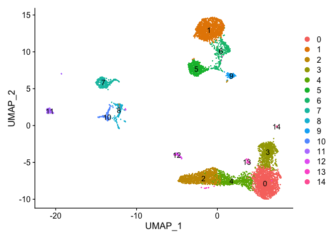
```r
DimPlot(s_balbc_pbmc, reduction = "umap", label = TRUE)
```
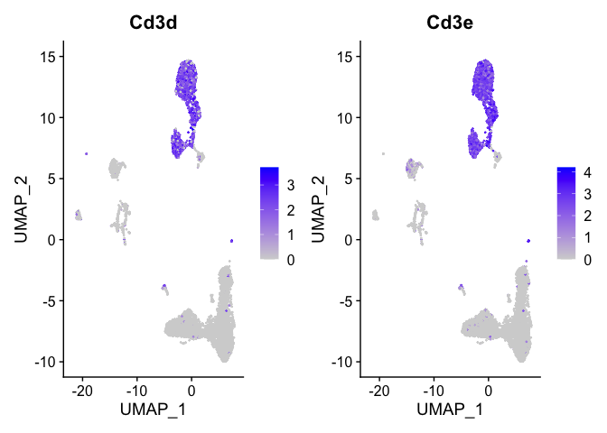
Lets look at T-cell and B-cell markers
```r
t_cell_markers <- c("Cd3d","Cd3e")
FeaturePlot(s_balbc_pbmc, features = t_cell_markers)
```

```r
table(!is.na(s_balbc_pbmc$t_clonotype_id),s_balbc_pbmc$seurat_clusters)
```
0 1 2 3 4 5 6 7 8 9 10 11 12 13
FALSE 1678 82 1174 807 656 47 37 326 176 149 132 125 44 35
TRUE 1 1337 0 0 0 455 312 6 9 5 2 8 13 6
14
FALSE 1
TRUE 11
```r
t_cells <- c("1","5","6")
```
Lets look at T-cell and B-cell markers
```r
t_cell_markers <- c("Cd3d","Cd3e")
FeaturePlot(s_balbc_pbmc, features = t_cell_markers)
```
```r
table(!is.na(s_balbc_pbmc$t_clonotype_id),s_balbc_pbmc$seurat_clusters)
```
0 1 2 3 4 5 6 7 8 9 10 11 12 13
FALSE 1678 82 1174 807 656 47 37 326 176 149 132 125 44 35
TRUE 1 1337 0 0 0 455 312 6 9 5 2 8 13 6
14
FALSE 1
TRUE 11
```r
t_cells <- c("1","5","6")
```
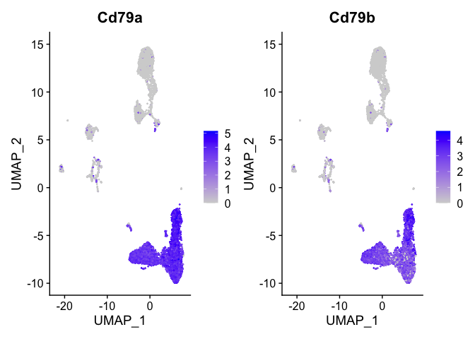
```r
b_cell_markers <- c("Cd79a","Cd79b")
FeaturePlot(s_balbc_pbmc, features = b_cell_markers)
```
```r
table(!is.na(s_balbc_pbmc$b_clonotype_id),s_balbc_pbmc$seurat_clusters)
```
0 1 2 3 4 5 6 7 8 9 10 11 12 13
FALSE 21 1417 1 4 2 501 347 306 161 138 122 116 21 7
TRUE 1658 2 1173 803 654 1 2 26 24 16 12 17 36 34
14
FALSE 12
TRUE 0
```r
b_cells <- c("0","2","3","4","12","13")
```
```r
markers_all = FindAllMarkers(s_balbc_pbmc,genes.use = VariableFeatures(s_balbc_pbmc),
only.pos = TRUE,
min.pct = 0.25,
thresh.use = 0.25)
```
Calculating cluster 0
For a more efficient implementation of the Wilcoxon Rank Sum Test,
(default method for FindMarkers) please install the limma package
--------------------------------------------
install.packages('BiocManager')
BiocManager::install('limma')
--------------------------------------------
After installation of limma, Seurat will automatically use the more
efficient implementation (no further action necessary).
This message will be shown once per session
Calculating cluster 1
Calculating cluster 2
Calculating cluster 3
Calculating cluster 4
Calculating cluster 5
Calculating cluster 6
Calculating cluster 7
Calculating cluster 8
Calculating cluster 9
Calculating cluster 10
Calculating cluster 11
Calculating cluster 12
Calculating cluster 13
Calculating cluster 14
```r
dim(markers_all)
```
[1] 6198 7
```r
head(markers_all)
```
p_val avg_logFC pct.1 pct.2 p_val_adj cluster gene
Fcer2a 0 1.499593 0.733 0.134 0 0 Fcer2a
H2-Ab1 0 1.269301 0.996 0.512 0 0 H2-Ab1
Ighd 0 1.260133 0.638 0.148 0 0 Ighd
H2-Aa 0 1.248650 0.999 0.515 0 0 H2-Aa
Mef2c 0 1.171142 0.822 0.425 0 0 Mef2c
H2-Eb1 0 1.141545 0.998 0.493 0 0 H2-Eb1
```r
table(table(markers_all$gene))
```
1 2 3 4 5 6 7 8
1580 690 467 271 108 23 5 5
```r
markers_all_single <- markers_all[markers_all$gene %in% names(table(markers_all$gene))[table(markers_all$gene) == 1],]
dim(markers_all_single)
```
[1] 1580 7
```r
table(table(markers_all_single$gene))
```
1
1580
```r
table(markers_all_single$cluster)
```
0 1 2 3 4 5 6 7 8 9 10 11 12 13 14
16 26 42 150 13 26 28 266 107 117 154 126 321 21 167
```r
head(markers_all_single)
```
p_val avg_logFC pct.1 pct.2 p_val_adj cluster gene
Fau 3.721948e-265 0.2935728 0.999 1.000 5.945811e-261 0 Fau
Fchsd2 3.324596e-229 1.0350500 0.532 0.201 5.311043e-225 0 Fchsd2
Rapgef4 8.954634e-106 0.6736929 0.304 0.109 1.430503e-101 0 Rapgef4
Lrrk2 1.155542e-77 0.5921848 0.267 0.106 1.845978e-73 0 Lrrk2
Pde4b 1.102262e-62 0.4857542 0.681 0.634 1.760863e-58 0 Pde4b
March1 7.301719e-58 0.6131182 0.320 0.181 1.166450e-53 0 March1
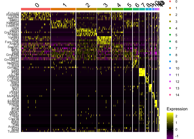
Plot a heatmap of genes by cluster for the top 5 marker genes per cluster
```r
library(dplyr)
```
Attaching package: 'dplyr'
The following objects are masked from 'package:stats':
filter, lag
The following objects are masked from 'package:base':
intersect, setdiff, setequal, union
```r
top5 <- markers_all_single %>% group_by(cluster) %>% top_n(5, avg_logFC)
dim(top5)
```
[1] 75 7
```r
DoHeatmap(
object = s_balbc_pbmc,
features = top5$gene
)
```
## Finally, save the object
```r
## Original dataset in Seurat class, with no filtering
save(s_balbc_pbmc,file="VDJ_object.RData")
```
## Session Information
```r
sessionInfo()
```
R version 4.0.0 (2020-04-24)
Platform: x86_64-apple-darwin17.0 (64-bit)
Running under: macOS Catalina 10.15.4
Matrix products: default
BLAS: /Library/Frameworks/R.framework/Versions/4.0/Resources/lib/libRblas.dylib
LAPACK: /Library/Frameworks/R.framework/Versions/4.0/Resources/lib/libRlapack.dylib
locale:
[1] en_US.UTF-8/en_US.UTF-8/en_US.UTF-8/C/en_US.UTF-8/en_US.UTF-8
attached base packages:
[1] stats graphics grDevices datasets utils methods base
other attached packages:
[1] dplyr_0.8.5 cowplot_1.0.0 Seurat_3.1.5
loaded via a namespace (and not attached):
[1] httr_1.4.1 tidyr_1.1.0 bit64_0.9-7 hdf5r_1.3.2
[5] jsonlite_1.6.1 viridisLite_0.3.0 splines_4.0.0 leiden_0.3.3
[9] assertthat_0.2.1 renv_0.10.0 yaml_2.2.1 ggrepel_0.8.2
[13] globals_0.12.5 pillar_1.4.4 lattice_0.20-41 glue_1.4.1
[17] reticulate_1.16 digest_0.6.25 RColorBrewer_1.1-2 colorspace_1.4-1
[21] htmltools_0.4.0 Matrix_1.2-18 plyr_1.8.6 pkgconfig_2.0.3
[25] tsne_0.1-3 listenv_0.8.0 purrr_0.3.4 patchwork_1.0.0
[29] scales_1.1.1 RANN_2.6.1 RSpectra_0.16-0 Rtsne_0.15
[33] tibble_3.0.1 farver_2.0.3 ggplot2_3.3.0 ellipsis_0.3.1
[37] withr_2.2.0 ROCR_1.0-11 pbapply_1.4-2 lazyeval_0.2.2
[41] survival_3.1-12 magrittr_1.5 crayon_1.3.4 evaluate_0.14
[45] future_1.17.0 nlme_3.1-148 MASS_7.3-51.6 ica_1.0-2
[49] tools_4.0.0 fitdistrplus_1.1-1 data.table_1.12.8 lifecycle_0.2.0
[53] stringr_1.4.0 plotly_4.9.2.1 munsell_0.5.0 cluster_2.1.0
[57] irlba_2.3.3 compiler_4.0.0 rsvd_1.0.3 rlang_0.4.6
[61] grid_4.0.0 ggridges_0.5.2 RcppAnnoy_0.0.16 htmlwidgets_1.5.1
[65] igraph_1.2.5 labeling_0.3 rmarkdown_2.1 gtable_0.3.0
[69] codetools_0.2-16 reshape2_1.4.4 R6_2.4.1 gridExtra_2.3
[73] zoo_1.8-8 knitr_1.28 bit_1.1-15.2 uwot_0.1.8
[77] future.apply_1.5.0 KernSmooth_2.23-17 ape_5.3 stringi_1.4.6
[81] parallel_4.0.0 Rcpp_1.0.4.6 vctrs_0.3.0 sctransform_0.2.1
[85] png_0.1-7 tidyselect_1.1.0 xfun_0.14 lmtest_0.9-37
