
Special Topics
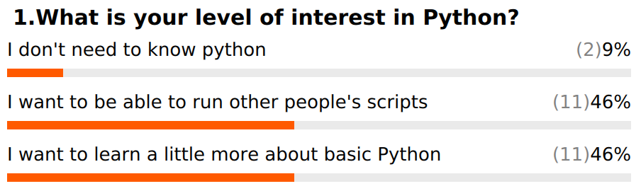
Based on our poll results, some people want more background on Python, while others are more interested in being able to install and use tools. We will try to address a bit more of both in this section.
Before we start, please log out of the server (ctrl+d or exit), then log back in to make sure that you have a clean new session.
Installing Software
Virtual Environments
Virtual environments give you the option to create a lightweight, self contained Python install where you can specify each module that is installed. This is a great option for keeping your system neat and tidy, and also keeps development versions of specific software isolated from your main Python library folders.
Another great thing about virtual environments is that you can use them to “snapshot” a set of modules for a project. As updates are released for these modules, the version you used for your project may become obsolete or unavailable. Keeping a virtual environment associated with the project ensures that you can always run the exact same versions of the software.
Python2 virtual environment and software install
Lets try it out by installing an older software package that hasn’t yet been updated to support Python3.
https://github.com/ibest/ARC
Log into the server and run the following commands.
run in bash $
# This path should have already been created, but we can make sure:
mkdir -p /share/workshop/prereq_workshop/$USER/python
cd /share/workshop/prereq_workshop/$USER/python

# Create the virtual environment:
virtualenv py2ARC.venv

# Activate virtual environment (note the change in your command prompt):
source /share/workshop/prereq_workshop/$USER/python/py2ARC.venv/bin/activate
At this point your bash prompt should start with (py2ARC.venv). If it does, click "Yes", if you are stuck click "No" or post a question on Slack.
Install software using pip and a setup.py build script for setuptools.
Installing biopython can take a little while. If you want you can learn what ARC does and review the installation instructions here.
run in bash $
# First we need to install dependencies:
# Biopython v1.76 was the last version released for Python 2.7.x
pip install biopython==1.76

# Clone a copy of the repository:
git clone https://github.com/ibest/ARC.git

# Install the software
cd ARC
python setup.py install


# Now you can test the install, but first we need to put a mapper and assembler in our path:
module load bowtie2
module load spades

cd test_data

ARC
At this point you should see a lot of text scrolling up the screen. This is ARC performing an iterative assembly process on some test data. If you see this, click "Yes", if you are stuck click "No" or post a question on Slack.
You can interrupt the assembly at any time using ctrl+c.
Once you are finished working in the Virtual Environment, you can exit it with the deactivate command. This will set your path and environment variables back to their normal state.
run in bash $
# Deactivate the virtual environment (look for a change in your prompt)
deactivate
Python3 virtual environment and software install (and using an API)
Python3 virtual environments are basically the same, but require slightly different commands.
Make sure that your python2 environment has been deactivated and then run the following.
run in bash $
# Make sure you are back in the right directory
cd /share/workshop/prereq_workshop/$USER/python

# We need a version of python3 that supports virtual environments.
source /share/biocore/shunter/opt/bin/setpath

# Create the python3 virtual environment, notice the difference in syntax.
python3 -m venv py3venv

# Activate the python3 virtual environment.
source py3venv/bin/activate
Note that if you get an error while creating the py3venv environment, you may have to delete it and try again after making sure to load the anaconda3 module.
At this point your bash prompt should start with (py3venv). If it does, click "Yes", if you are stuck click "No" or post a question on Slack.
Now we are ready to install modules into our Python3 virtual environment. Lets try out the covid package to query data on the novel corona virus.
To do this we will use pip, the package installer for Python. Pip will automatically download and install all of the dependencies needed for the covid package.
Again, this process might take a little while, so while you wait, visit the covid package page, scroll down to the “How to use” section of the page and review the usage instructions. The covid package installs includes a command line tool written in Python (you can look at some of the source code using less ./py3venv/lib/python3.6/site-packages/covid/cli.py). Try to determine the number of confirmed cases based on worldometers and john_hopkins data sources. Are they the same?
run in bash $
# Installing is easy, just use pip!

pip install covid

# Once the install has finished, run python:
python
Try running the following code to fetch the latest data on Italy. What kind of data type does get_status_by_country_name() return? You should be able to access elements of the dataset using information from yesterday’s course material.
run in python »>
from covid import Covid

covid = Covid()


covid.get_status_by_country_name("italy")
Once you are finished, remember that you can exit Python using ctrl+D, and use deactivate to exit from the Python3 virtual environment.
Bonus Exercise:
1) MultiQC support for our Illumina read QA/QC etc application HTStream is almost complete. However, it has not been merged in to the official MultiQC repository yet. The only way to get it is to install it yourself from https://github.com/s4hts/MultiQC. Using what you have learned so far, try to install this version of MultiQC in your Python3 virtual environment. * Once you have the multiqc package installed, you can get some test data to try on using the following commands.
wget "https://raw.githubusercontent.com/ucdavis-bioinformatics-training/2020-Bioinformatics_Prerequisites_Workshop/master/Intro_to_Python/multiqcData.tar.gz"

tar xvf multiqcData.tar.gz
Break
Basic File Operations
Reading and writing files in Python is easy with built in support for common operations.
In order to work with a file, we send a request to the operating system to open a handle to the file. This handle allows us to send and/or receive information from the file depending on what mode we open the file in.
The steps are: 1) Open a file handle. 2) Read or write data. 3) Close file handle.
Writing to a file:
run in bash $
# Make sure you are back in the right directory
cd /share/workshop/prereq_workshop/$USER/python

# First, make sure that a more recent version of python is available:
source /share/biocore/shunter/opt/bin/setpath
NOTE we need python 3.8 to run the code below
run in python »>
# 1) Open a file handle to write text to:
handle = open("test_file.txt", "w")

# 2) Lets practice looping over a range of integers and writing them to our file:
for i in range(0,20):
    handle.write(f"Integer {i}\n")

# 3) Close the file handle
handle.close()

# If you are running ipython try "cat test_file.txt" to check the contents of the file.
# If you are not running ipython, either connect to the server in another terminal
# window to look at the contents of the file, or exit from python, cat the file and start python again.
Reading from a file:
Now lets reverse the process and read the information back in from the file.
This time we will try at a few alternative approaches.
The first two automatically close the file for us when we are done because we use the with statement.
The final example shows how to manually read one line from the file with the next() method. Note that the file handle is an iterable object. The next() statement can be used to request the next line from a file handle iterator (the file handle is technically an iterable object AND an iterator). In the first example, the for loop calls next() over and over, storing the resulting value in a variable called line that we use in the print() statement.
run in python »>
# Option 1, iterates over the file line by line:
with open("test_file.txt", "r") as handle:
    for line in handle:
        print(line.strip())

# Option 2, reads the entire file in and prints it
with open("test_file.txt", "r") as handle:
    print(handle.read())

# Bonus: What if we want to look at the file manually one line at a time?
handle = open("test_file.txt", "r")
line = next(handle)
print(line)
handle.close()
What about compressed files?
Many algorithms have been developed for reducing the size of a file by taking advantage of short repeated sections of a file. For example, imagine we had some data like: “AAAAAAGGGGGGGTTTTTTTTCCCCCCCCC”, we could encode this value as “A6G7T8C9” and save a lot of space! This approach to data compression is called Run Length Encoding or RLE and is sometimes used with Oxford Nanopore and PacBio CLR data to overcome problems with homopolymers.
In this example we will use a file that is compressed with a more complex algorithm that is commonly used for storing files on Linux called gzip.
First we need a compressed file to work with, we will use a module called urllib.request to download the file from GitHub, and the os module to perform so tests on the file to see if it downloaded properly.
run in python »>
import urllib.request
url = "https://raw.githubusercontent.com/ucdavis-bioinformatics-training/2020-Bioinformatics_Prerequisites_Workshop/master/Intro_to_Python/example_data.fastq.gz"

urllib.request.urlretrieve(url, 'example_data.fastq.gz')


# Use more functions in os to check on the download:
import os
os.path.isfile("example_data.fastq.gz")

os.path.getsize("example_data.fastq.gz")

# If you are running ipython, try "less -S example_data.fastq.gz" to get a look at the file.
The file we just download is a FastQ formatted file, containing data from an Illumina MiSeq sequencer. If you look closely, you will see that each record is made up of four lines. You will learn more about this file type later in the workshop.
1) The first line starts with “@” and contains the Read ID. 2) The second line contains the actual sequence data (ACGT or N). 3) The third line is a “+” sign, and in some older files also contains the Read ID. 4) The fourth line contains an ASCII encoding of the Phred + 33 quality score.
@M02034:434:000000000-CHDFR:1:1101:13812:1361
AGGGAATCTTCCGCAATGGACGAAAGTCTGACGGAGCAACGCCGCGTGAGTGATGAAGGTTTTCGGATCGTAAAGCTCTGTTGTTAGGGAAGAACAAGTACCGTTCGAATAGGGCGGTACCTTGACGGTACCTAACCAGAAAGCCACGGCTAACTACGTGCCAGCAGCCGCGGTAATACGTAGGTGGCAAGCGTTGTCCGGAATTATTGGGCGTAAAGGGCTCGCAGGCGGTTCCTTAAGTCTGATGTGAAAGCCCCCGGCTCAACCGGGGAGGGTCATTGGAAACTGGGGAACTTGAGTGCAGAAGAGGAAAGTGGAATTCCATGTGTAGCGGTGAAATGCGCAGAGATATGGAGGAACACCAGTGGCGAAGGCGACTTTCTGGTCTGTAACTGACGCTGATGTGCGAAAGCGTGGGGATCAAACAGG
+
GGGGGGGGGGGGGGGGGGGFGGFGGGGGGGGGGGGGGGGGGGGGGGFGGGGGGGGGGGGGGGGGGGGGGGGGGGGGGGGGGGGGGGGGGGGGGFFFGGGGGGGFGGGGGGGGGGGGEFGGGGGGCFGDGGGGGGGGGGGGGGGGGGGGGGGGGGIIIIIIIIIIIIIIIIIIIIIIIIIIIIIIIIIIIIIE?IIIIIIIIII6IIIIIIIIIIIIIIIIIGI:<EEIIIIIIIIIIIIIIF"DIIIIIIIIIIIIIIIIIIIIIIIIIIIIIII+CF9GGGFGEGGFFGGGFGGGFGGFGCGGGGGGGGGFFGGGFDGFFGCEEGGEEGGGGGGGGEFDGGFFGGGGGGGGGGFGGGGGFDEFGGGGFGEGGFDGGGFFGGGGGGFFGGFGDGGGGGGGGGGGGGGGGGGGGGGGGFGGGGGGGGGGG
@M02034:434:000000000-CHDFR:1:1101:9702:6439
AGGGAATCTTCCGCAATGGACGAAAGTCTGACGGAGCAACGCCGCGTGAGTGATGAAGGTTTTCGGATCGTAAAGCTCTGTTGTTAGGGAAGAACAAGTACCGTTCGAATAGGGCGGTACCTTGACGGTACCTAACCAGAAAGCCACGGCTAACTACGTGCCAGCAGCCGCGGTAATACGTAGGTGGCAAGCGTTGTCCGGAATTATTGGGCGTAAAGGGCTCGCAGGCGGTTCCTTAAGTCTGATGTGAAAGCCCCCGGCTCAACCGGGGAGGGTCATTGGAAACTGGGGAACTTGAGTGCAGAAGAGGAGAGTGGAATTCCACGTGTAGCGGTGAAATGCGTAGAGATGTGGAGGAACACCAGTGGCGAAGGCGACTCTCTGGTCTGTAACTGACGCTGAGGAGCGAAAGCGTGGGGAGCGAACAGG
+
GGGGGGGGGGGGGGGFGGGGGGGGGGGGGGGGGGGGGGGGGGGEGGGGGGGGGGGGGGGGGGGGGGGGGGGGGGGGFGGAFGGGGGGGGGGGGGGGGGGGGGGGGGGGGGGGGGGGGGGGGGGGGGGGGGGGGGGGGGGGGGGGGGFGEGGGIIIIIIIIIIIIIIIIIIIIIIIIIIIIIIII?IIIIIIIIIIIIIIIIIIIIIIIIIIIIIIIIIIIIIIIIIIIIII"IIIIIIIIIIIIIIIIIIIIIIIIIIIIIIIIIIIIIIIIIIIIIIEIIFDBDDGGGFD=DCGGGFGGGDGGGGGGFFAGGGGGGGFGGECGGGECEGE7GFFGAEEGGGGGGFAGEFGFGFDEFCEDCCFGGCGGFFGGGGGGGDGGGFGGGGGGGGGGGGGGGGGGGGGGEGGGFFGGGGGGGGGGGGGGGGGFF
@M02034:434:000000000-CHDFR:1:1101:21100:7204
AGGGAATCTTCCGCAATGGACGAAAGTCTGACGGAGCAACGCCGCGTGAGTGATGAAGGTTTTCGGATCATAAAGCTCTGTTGTTAGGGAAGAACAAGTACCGTTCGAATAGGGCGGTACCTTGACGGTACCTAACCAGAAAGCCACGGCTAACTACGTGCCAGCAGCCGCGGTAATACGTAGGTGGCAAGCGTTGTCCGGAATTATTGGGCGTAAAGGGCTCGCAGGCGGTTCCTTAAGTCTGATGTGAAAGCCCCCGGCTCAACCGGGGAGGGTCATTGGAAACTGGGGAACTTGAGTGCAGAAGAGGAGAGTGGAATTCCACGTGTAGCGGTGAAATGCGTAGAGATGTGGAGGAACACCAGTGGCGAAGGCGACTCTCTGGTCTGTAACTGACGCTGAGGAGCGAAAGCGTGGGGAGCGAACAGG
+
GGGGGGGGGGGGGGGGGGGGGGGGGGGGGGGGGGGGGGGGGGGGGGGGGGGGGGGGGGGGGGGGCGGGGGGGGGGGGGGGGGGFFGGGGFGGGGGGGGGGGGGEGFGGGGGGGGGGGGGGGGGGGGGGGGGGGFGGGGGGGGEGGFGGGGGGGI"IIIIIIIIIIIIIIIIIIIIIIIIIIIIIIIIIIIIIIII""IIIIIIIIIIIIIIIIIIIIIIIIIIIIIIIIIII2IIIIIIIIIIIIIIIIIIIIIIIIIIIIIIIIIIIIII$AIIGGGGFDGGGGCFGFFGGGGGFFDGFCGGGGFFFGGGGFE,GGGGGGGFEFGFEGGECGGGDGGGGGFFAGGDGGGFGGGGGGGGGFCGGF7GGGGGGGGFF?GGGGGFGGFGGGGGGGGGGGGGGFFEGGGDGGGGGGGGGGGGGGGGGGGGGF
If we try to open this file like we did with the previous file we will get incomprehensible garbage. In order to read the file properly, we need to uncompress it. The Python gzip module allows us to do this, but otherwise works like the normal file handle. Note that we open the file in “rt”, or read-text mode.
run in python »>
import gzip

# Note that 'rt' opens the file for text reading
handle = gzip.open("example_data.fastq.gz", 'rt')

l = next(handle)

print(l)

handle.close()
Lets pretend that for some reason we want to process the whole file and count how many times we see each character? Can you figure out how this code works?
Hints: 1) Remember, h is a gzip file handle iterator that will return one line at a time. 2) line.strip() removes special characters and for ch in line.strip() iterates over each character.
run in python »>
import gzip
# Create an empty dictionary
chrcount = {}

# read in each line of the fasta file, count character occurrences
with gzip.open('example_data.fastq.gz', 'rt') as h:
    for line in h:
        for ch in line.strip():
            if ch not in chrcount:
                chrcount[ch] = 0
            chrcount[ch] += 1

# Print out the character (dictionary key) and associated value (the count):
for k, v in chrcount.items():
    print(f"character:{k}, count:{v}")
Sorting in Python
We might want to print out values from most common to least. To do this, we need a way to sort. Python has a built in sorted() function that can take care of this for us. The sorted() function is a little bit tricky because the “key” argument has to be a function. This is very powerful because it allows flexibility, but can also be confusing.
Try to figure out how the call to sorted() works.
Some Hints: 1) What does chrcount.items() return? 2) What does x and x[1] contain if you run this code: x = list(chrcount.items())[0]?
run in python »>
# Check how sorted works:
sorted([4,2,5,6,2])

#
sorted([4,2,5,6,2], reverse=True)

# Sorting your dictionary by value requires some tricks:
sorted(chrcount.items(), key=lambda x: x[1], reverse=True)

# The lambda keyword allows us to create a function "on the fly". The
# following code shows how this works.
def getv(x):
    return(x[1])

sorted(chrcount.items(), key=getv, reverse=True)
Exercises
-
Try to open the example_data.fastq.gz file without using gzip. Read the first line into a variable called “l”, then print it. What happens?
-
How many base pairs long is the first read in the file?
- The ord() function will return the ASCII value for a single character. Write some code to read the fourth line from the fastq file, then covert the values to a quality score and calculate the average quality value.
- Hints: The last character is a line return (\n), use strip() to remove it. You can use list comprehension or a for loop to split up the characters and run ord() on each one.
- Write some code to figure out how many total lines are in example_data.fastq.gz. How many reads is this?
Once you have successfully completed the exercises, mark "Yes" in zoom. Post questions or problems to the Slack channel.
Break
BioPython
![]()
Biopython is an open source collection of tools for manipulating biological data. The types of data it supports and operations it provides for these data types are documented in the Biopython Tutorial and Cookbook and are quite extensive.
Before we start we need to ensure that the BioPython module is loaded. On the bash command line load the biopython module and then run python3.
run in bash $
# Make sure you are back in the right directory
cd /share/workshop/prereq_workshop/$USER/python

module load biopython
python3
Explore Biopython Sequence objects
run in python »>
from Bio.Seq import Seq

# Create a Seq object:
m = Seq("AGTCCGTAG")

# Normal string indexing still work
print(m[0])

# Slicing still works, get the first two letters:
m[:2]

# And the last two:
m[-2:]

# Print the Positive and Negative number index
for index, letter in enumerate(m):
    print(f"{index} {index - len(m)} {letter}")

# In some cases sequences may need to be upper/lower case:
m.lower()

m.upper()

# Characters can be counted just like with strings:
100 * (m.count('C') + m.count('G')) / len(m)

# We can even join two Seq() objects, or a Seq() and a String:
n = m + "AAAAAAAAAAA"

print(n)

# However Seq objects also support a number of useful functions:
m.reverse_complement()

m.translate(table=11)
SeqIO provides an interface to read/write a large number of different Bioinformatics file formats.
Using SeqIO should look very familiar after learning about file handles. Note that we need to provide a file type so that SeqIO knows how to properly read our file.
run in python »>
# Import SeqIO module
from Bio import SeqIO

# Create  a gzip file handle
handle = gzip.open("example_data.fastq.gz", 'rt')

# Tell SeqIO to parse the data in the file in fastq format
parser = SeqIO.parse(handle, 'fastq')

# Extract the first record
record = next(parser)

# Explore the record object:
record.id

record.seq

len(record)

# Calculate average quality score
sum(record.letter_annotations['phred_quality'])/len(record)
Use SeqIO to get the lenths of all sequences in the file and calculate statistics.
run in python »>
from Bio import SeqIO
import gzip
import statistics

with gzip.open("example_data.fastq.gz", 'rt') as h:
    l = [len(r) for r in SeqIO.parse(h, 'fastq')]


max(l)

min(l)

sum(l)/len(l)

# How many reads are < 427bp?
sum(m < 429 for m in l)

sum(m > 429 for m in l)
Another common use of SeqIO is to convert from one file type to another:
run in python »>
from Bio import SeqIO
import gzip

with gzip.open("example_data.fastq.gz", 'rt') as inf, gzip.open("example_data.fasta.gz", 'wt') as outf:
    SeqIO.convert(inf, "fastq", outf, "fasta")

# If you are running ipython, use less to check whether the file has been converted.
Break
CSV package
It is commonly necessary to read or write tabular data when doing bioinformatics work. Python has a handy module to support this called CSV.
Lets experiment with writing and reading tabular files using the DictWriter and DictReader classes.
run in python »>
# Write a tab-separated values file with
import csv

# First lets write an example file
with open('my_data.csv', 'w') as csvfile:
    # Create a list with the column headers
    fieldnames = ['SampleID','Age','Treatment', 'Weight']
    # Create a DictWriter, use tabs to delimit columns
    writer = csv.DictWriter(csvfile, fieldnames=fieldnames, delimiter='\t')
    # Write out the header
    writer.writeheader()

    writer.writerow({"SampleID":"mouse1", "Age":4, "Treatment":"Control", "Weight":3.2})
    writer.writerow({"SampleID":"mouse2", "Age":5, "Treatment":"Control", "Weight":3.6 })
    writer.writerow({"SampleID":"mouse3", "Age":4, "Treatment":"Control", "Weight":3.8 })
    writer.writerow({"SampleID":"mouse4", "Age":4, "Treatment":"ad libitum", "Weight":3.6 })
    writer.writerow({"SampleID":"mouse5", "Age":4, "Treatment":"ad libitum", "Weight":3.7 })
    writer.writerow({"SampleID":"mouse6", "Age":4, "Treatment":"ad libitum", "Weight":3.5 })

# If you are running ipython, try checking the contents of the file with "cat my_data.csv"
run in python »>
# Reading data in from a file and print it to the screen
import csv

with open('my_data.csv', 'r') as csvfile:
    reader = csv.DictReader(csvfile, delimiter='\t')
    for row in reader:
        print(f"SampleID:{row['SampleID']}, Age:{row['Age']}, Treatment:{row['Treatment']}, Weight:{row['Weight']}")
Exercises
-
Use SeqIO to filter the records in from example_data.fastq.gz. Create a new file called data_filtered.fastq. Only write reads that DO NOT start with “AGGG”. How many reads were there?
-
Use SeqIO and the CSV package to record statistics for the reads in example_data.fastq.gz. Create a CSV file called read_stats.tsv. Create a DictWriter with column names: (ReadID, Length, GCcontent, AverageQuality). Collect each of these pieces of information for each read, and write it to the CSV file.
-
Use SeqIO and a Dictionary, count the frequency of the first 15bp and last 15bp of each read in example_data.fastq.gz. What are the most common sequences?
-
Using the covid module, download the latest data and export it to a CSV file. Save a copy somewhere and make some informative plots using R later in the week.
Once you have successfully completed the exercises, mark "Yes" in zoom. Post questions or problems to the Slack channel.
Wrapping up
- Learning a new programming language takes time and patience. This rapid overview may have felt overwhelming, especially if you haven’t programmed before. That is pretty normal.
- Keep practicing, hands-on programming is the only way to learn. A great option is to just “play” and see what happens.
- Employ the Scientific Method: 1) Form a hypothesis about how Python works, 2) Design an experiment to test your hypothesis, 3) Reject or accept your hypothesis depending on the results.
- There are a nearly overwhelming number of free tutorials online. Working through these tutorials is a great way to keep learning.
-
Many of the ideas we discussed today are common to most programming languages, even if some details of syntax differ. During the intro to R section, look for similarities (and differences). If you understand the concepts, you can always Google for syntax.
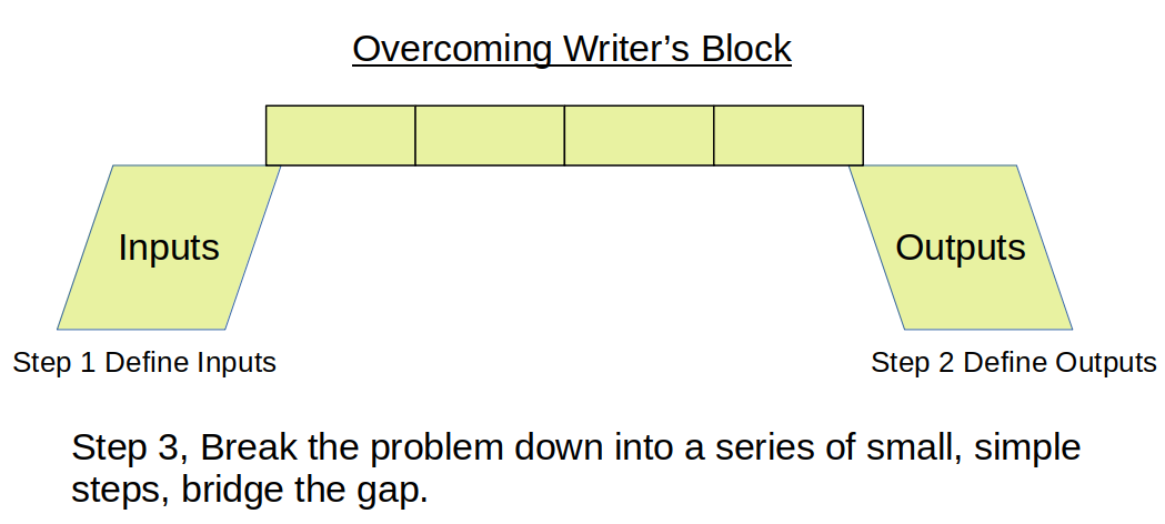
- If you get stuck solving a problem, try to break it down into a set of simple steps.
- Define (write down) your inputs.
- Define (write down) your outputs.
- Once you have inputs and outputs defined, you often will see a path to the solution.
- If not, look for a first simple step (e.g. How should I load the data?, How should I store the data?).
- Continue to identify steps that lead you towards the set of outputs you defined.
- Each of these steps will help you understand your data and the problem better, and eventually help you find the path to a solution.
Additional things to check out (but mostly just Google everything)
https://biopython.org/DIST/docs/tutorial/Tutorial.html
https://realpython.com/
https://seaborn.pydata.org/
http://ggplot.yhathq.com/